Travel Graphs
This section covers travel graphs, speed, distance, time, trapezium rule and velocity.
Speed, Distance and Time
The following is a basic but important formula which applies when speed is constant (in other words the speed doesn't change):
Remember, when using any formula, the units must all be consistent. For example speed could be measured in m/s, distance in metres and time in seconds.
If speed does change, the average (mean) speed can be calculated: Average speed = total distance travelled total time taken
In calculations, units must be consistent, so if the units in the question are not all the same (e.g. m/s, m and s or km/h, km and h), change the units before starting, as above.
The following is an example of how to change the units:
Change 15km/h into m/s. 15km/h = 15/60 km/min (1) = 15/3600 km/s = 1/240 km/s (2) = 1000/240 m/s = 4.167 m/s (3)
In line (1), we divide by 60 because there are 60 minutes in an hour. Often people have problems working out whether they need to divide or multiply by a certain number to change the units. If you think about it, in 1 minute, the object is going to travel less distance than in an hour. So we divide by 60, not multiply to get a smaller number.
If a car travels at a speed of 10m/s for 3 minutes, how far will it travel? Firstly, change the 3 minutes into 180 seconds, so that the units are consistent. Now rearrange the first equation to get distance = speed × time. Therefore distance travelled = 10 × 180 = 1800m = 1.8km
Velocity and Acceleration
Velocity is the speed of a particle and its direction of motion (therefore velocity is a vector quantity, whereas speed is a scalar quantity).
When the velocity (speed) of a moving object is increasing we say that the object is accelerating . If the velocity decreases it is said to be decelerating. Acceleration is therefore the rate of change of velocity (change in velocity / time) and is measured in m/s².
A car starts from rest and within 10 seconds is travelling at 10m/s. What is its acceleration?
Distance-Time Graphs
These have the distance from a certain point on the vertical axis and the time on the horizontal axis. The velocity can be calculated by finding the gradient of the graph. If the graph is curved, this can be done by drawing a chord and finding its gradient (this will give average velocity) or by finding the gradient of a tangent to the graph (this will give the velocity at the instant where the tangent is drawn).
Velocity-Time Graphs/ Speed-Time Graphs
A velocity-time graph has the velocity or speed of an object on the vertical axis and time on the horizontal axis. The distance travelled can be calculated by finding the area under a velocity-time graph. If the graph is curved, there are a number of ways of estimating the area (see trapezium rule below). Acceleration is the gradient of a velocity-time graph and on curves can be calculated using chords or tangents, as above.
The distance travelled is the area under the graph. The acceleration and deceleration can be found by finding the gradient of the lines.
On travel graphs, time always goes on the horizontal axis (because it is the independent variable).
Trapezium Rule
This is a useful method of estimating the area under a graph. You often need to find the area under a velocity-time graph since this is the distance travelled.
Area under a curved graph = ½ × d × (first + last + 2(sum of rest))
d is the distance between the values from where you will take your readings. In the above example, d = 1. Every 1 unit on the horizontal axis, we draw a line to the graph and across to the y axis. 'first' refers to the first value on the vertical axis, which is about 4 here. 'last' refers to the last value, which is about 5 (green line).] 'sum of rest' refers to the sum of the values on the vertical axis where the yellow lines meet it. Therefore area is roughly: ½ × 1 × (4 + 5 + 2(8 + 8.8 + 10.1 + 10.8 + 11.9 + 12 + 12.7 + 12.9 + 13 + 13.2 + 13.4)) = ½ × (9 + 2(126.8)) = ½ × 262.6 = 131.3 units²


Ultimate Guide to Travel Graphs| Cambridge IGCSE Mathematics
Kulni gamage.
- Created on July 20, 2023
[Please watch the video attached at the end of this blog for a visual explanation on the Ultimate Guide to Travel Graphs]
Travel graphs fall under the bigger topic of Algebra, but unlike the other lessons under this topic, this is really simple and easy to understand… as long as you read the question carefully and pay attention to the readings of the graphs ?!
What is a travel graph?
A travel graph is a line graph that tells us how much distance has been covered by the object in question within a particular time. We can use travel graphs to represent the motion of cars, people, trains, buses, etc. This means travel graphs can tell us whether an object is still (stationary), moving at a constant speed, accelerating, or decelerating. The y -axis represents the distance travelled while the x -axis shows the time it takes to travel a distance such as that.
James went on a cycling ride. The travel graph shows James’s distance from home on this cycle ride. Find James’s speed for the first 60 minutes.
We are told that James is going on a cycling ride and that the distance he travelled is what is shown here. What is required of us is to find James’s speed for the first 60 minutes. This means you need to mark the point at 60 minutes on the x -axis as shown in the picture below.
We have learnt when learning about Speed, Time and Distance that speed = distance/ time.
Therefore, in a distance-time graph, the slope that we see (also called the gradient) is what will give us the speed.
We can see that this particular cycle has travelled 12 km in 60 minutes.
When we substitute these values into the formula above, it would look like this:
When this formula is solved, then we get James’s speed for the first 60 minutes , which is 0.2 km/min .
A train journey takes one hour. The diagram shows the speed-time graph for this journey. Calculate the total distance of this journey.
We need to be careful here because this time what we have in this question is a speed-time graph and not a distance-time graph.
In a speed-time graph, the gradient of a slope represents either acceleration or deceleration, which will be concepts touched upon in later lessons. The distance travelled is found by calculating the area under a speed-time graph.
In order to calculate the distance travelled by the train therefore, we need to calculate the area under the graph that is drawn. To make things easier, we can separate this graph into shapes:
2 triangles and 1 rectangle
Triangle 1: Area of a triangle = ½ × base of triangle × height of triangle Area = ½ × 4 km × 3 km/min Area = 6 km2
Rectangle: Length of the rectangle can be found by finding out the difference between 50 and 4, which equals to 46 min. The height of the rectangle is 3 km/min. Area = length × base Area = 46 min × 3 km/min Area = 138 km
Triangle 2: Area of a triangle = ½ × base of triangle × height of triangle Area = ½ × 10 km × 3 km/min Area = 15 km
Total Area under the graph = Total distance travelled by the train Therefore, Total Distance = Triangle 1 + Rectangle + Triangle 2 Total Distance = 6 km + 138 km + 15 km Total Distance = 159 km
Those are the basic tips and tricks you would need to learn in this particular chapter!
Travel Graphs at Exams
Pay attention to what sort of graph is given to you. Is it a distance-time graph? A speed-time graph? Depending on the type of graph, remember, the value represented by the gradient changes, and so does the value represented by the area under the graph.
Practice as many questions as you can on this topic. They are quite simple once you get the hang of them. You can find some questions in this quiz to check where you stand!
If you are struggling with IGCSE revision or the Mathematics subject in particular, you can reach out to us at Tutopiya to join revision sessions or find yourself the right tutor for you.
Watch the video below for a visual explanation of the lesson on the ultimate guide to travel graphs!
See author's posts
Recent Posts
- IGCSE Exam 2024 Revision: 10 Tips and Tricks to Score A*
- How to Ace Your IGCSE Exam in 3 Months: A Comprehensive Guide to Score A*
- Tutopiya’s Shining Star: An Insight into the Teaching Journey of Anshu Gupta
- IGCSE Group Classes in Singapore: Exam Preparation, Pricing, Benefits and Online Resources
- 1:1 IGCSE Online Tutoring in Malaysia: Benefits, Challenges, Online Resources and How to Succeed
- IGCSE Mock Assessment: Prepare with Tutopiya’s Practice Exams
- IGCSE Online Tutors Dubai: Boost Your Grades Now
- How to Stay Calm and Confident in IGCSE Exams
- Avoid These 7 Common IGCSE Exam Mistakes for Better Grades: Tutopiya
- IGCSE in Singapore: Expat Guide to Top Education & Tutopiya’s Support
Get Started
Learner guide
Tutor guide
Curriculums
IGCSE Tuition
PSLE Tuition
SIngapore O Level Tuition
Singapore A Level Tuition
SAT Tuition
Math Tuition
Additional Math Tuition
English Tuition
English Literature Tuition
Science Tuition
Physics Tuition
Chemistry Tuition
Biology Tuition
Economics Tuition
Business Studies Tuition
French Tuition
Spanish Tuition
Chinese Tuition
Computer Science Tuition
Geography Tuition
History Tuition
TOK Tuition
Privacy policy
22 Changi Business Park Central 2, #02-08, Singapore, 486032
All rights reserved
©2022 tutopiya
| Home Page | Order Maths Software | About the Series | Maths Software Tutorials | | Year 7 Maths Software | Year 8 Maths Software | Year 9 Maths Software | Year 10 Maths Software | | Homework Software | Tutor Software | Maths Software Platform | Trial Maths Software | | Feedback | About mathsteacher.com.au | Terms and Conditions | Our Policies | Links | Contact |
Copyright © 2000-2022 mathsteacher.com Pty Ltd. All rights reserved. Australian Business Number 53 056 217 611
Copyright instructions for educational institutions
Please read the Terms and Conditions of Use of this Website and our Privacy and Other Policies . If you experience difficulties when using this Website, tell us through the feedback form or by phoning the contact telephone number.

Visual maths worksheets, each maths worksheet is differentiated and visual.
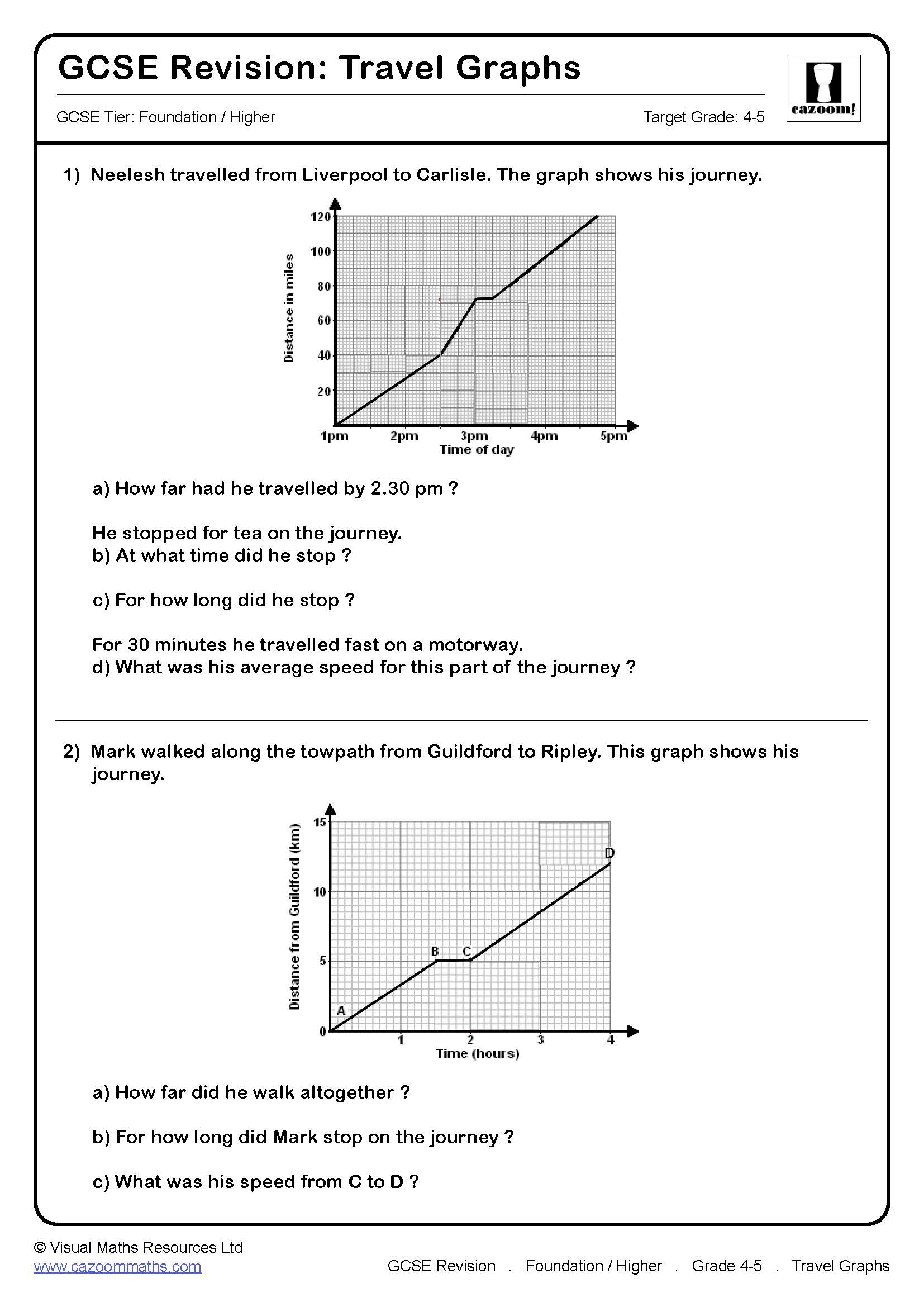
Travel Graphs GCSE Questions PDF
Total reviews: (0), travel graphs gcse revision description.
This set of questions provides travel graphs in the form of distance-time graphs. Learners will need to read information from the graphs, such as distances at certain times and periods of rest. They will also need to calculate the speed between different times.
WE LOVE TO GET YOUR FEEDBACK:
🐣📚 EGGCITING EASTER MATHS WORKSHEETS 🐰✏️ DOWNLOAD NOW! 🎉
Thank you for submitting the form
Get 20 FREE MATHS WORKSHEETS
Fill out the form below to get 20 FREE maths worksheets!

TOM ROCKS MATHS
Maths, but not as you know it…, gcse maths: travel graphs (speed-distance-time).
Learn how to use travel graphs relating speed, distance and time to solve problems. Tom introduces the topic, Bobby applies it to Usain Bolt’s 100-metre world record, and Susan uses an interactive tool on GeoGebra – go to www.geogebra.org/m/ABuBYdX7 to join in at home.
This is the second lesson in a new series with the Maths Appeal duo – Bobby Seagull and Susan Okereke – and Tom Rocks Maths where we’ll be exploring the GCSE Maths syllabus to show the world that maths is accessible to everyone!
Watch Bobby and Susan answer YOUR questions here .
Watch Tom’s livestream here .
Share this:
- Click to share on Twitter (Opens in new window)
- Click to share on Facebook (Opens in new window)
- Click to share on Reddit (Opens in new window)
- Click to share on LinkedIn (Opens in new window)
- Click to email a link to a friend (Opens in new window)
- Click to share on Pinterest (Opens in new window)
- Click to share on WhatsApp (Opens in new window)
- Click to share on Tumblr (Opens in new window)
[…] Watch the video for lesson 2 (Travel graphs) here. […]
[…] Watch the video lesson here. […]
Leave a comment Cancel reply

- Already have a WordPress.com account? Log in now.
- Subscribe Subscribed
- Copy shortlink
- Report this content
- View post in Reader
- Manage subscriptions
- Collapse this bar
Transum Shop :: Laptops aid Learning :: School Books :: Tablets :: Educational Toys :: STEM Books
Menu Level 1 Level 2 Level 3 Level 4 Exam Help More Graphs
This is level 4; Draw a travel graph from the given description. Click on the points at the ends of where the straight line segments of the graphs should be.
This is Travel Graphs level 4. You can also try: Level 1 Level 2 Level 3

For Students:
- Times Tables
- TablesMaster
- Investigations
- Exam Questions

For Teachers:
- Starter of the Day
- Shine+Write
- Breaking News
- Random Names
- Maths Videos
- Laptops in Lessons
- Maths On Display
- Class Admin
- Create An Account
- About Transum
- Privacy Policy
©1997-2024 WWW.TRANSUM.ORG
Description of Levels
Level 1 - Reading information from distance-time graphs
Level 2 - Matching distance-time graphs with their descriptions
Level 3 - Reading information from speed-time graphs
Level 4 - Draw a travel graph from the given description
Exam Style Questions - A collection of problems in the style of GCSE or IB/A-level exam paper questions (worked solutions are available for Transum subscribers).
More Graphs including lesson Starters, visual aids, investigations and self-marking exercises.
Answers to this exercise are available lower down this page when you are logged in to your Transum account. If you don’t yet have a Transum subscription one can be very quickly set up if you are a teacher, tutor or parent.
Log in Sign up
Distance-Time Graphs
For a basic introduction to distance-time graphs see Hurdles Race . For more details play the video below.
Don't wait until you have finished the exercise before you click on the 'Check' button. Click it often as you work through the questions to see if you are answering them correctly. You can double-click the 'Check' button to make it float at the bottom of your screen.
NESA is regularly updating its advice as the coronavirus outbreak unfolds. Get our latest COVID-19 advice
This webpage has been archived to prepare for transfer to the new NESA website . Reference to syllabus outcomes and content on this webpage may not be current. Teachers are encouraged to visit the Key Learning Area page for recent student work samples on the NESA website .
Assessment Resource Centre (ARC)
- NSW Government
- ABOUT BOSTES
- Years 11-12
- Mathematics
- Work Samples
- Can-do Trigonometry
- Using Histograms and Polygons
- Best Airfare Deals
- Probability
- Successive Discounts
- Draw the Graph to Fit the Story
- Similar? Congruent?
- The Pyramid of Giza
- Graphs of Relationships
- Simultaneous Equations
- Additional Information
- Surface Area and Volume
- Applications of Simple and Compound Interest
Areas for Assessment
Describing travel graphs, description of activity.
For each of the six travel graphs, students will be asked to write a brief description of the journey that the graph might represent.
Students will complete the accompanying worksheet.
Patterns and Algebra, Working Mathematically
This assessment activity could be presented to students during, or at the end of, a unit on Graphs of Physical Phenomena, where students have been drawing and interpreting a variety of travel graphs, as well as providing descriptions of the meanings of different gradients for graphs of particular events.
- Working mathematically Knowledge, skills and understanding developed through inquiry, application of problem-solving strategies, communication, reasoning and reflection
- Patterns and algebra Knowledge, skills and understanding in patterning, generalisation and algebraic reasoning
Graphs of Physical Phenomena (PAS5.2.5) Draws and interprets graphs of physical phenomena
Applying Strategies (WMS5.2.2) Selects and uses appropriate problem-solving strategies that include selecting and organising key information and identifying and working on related problems
Communicating (WMS5.2.3) Uses appropriate mathematical language and algebraic, statistical and other notations and conventions in written, oral or graphical form
Reasoning (WMS5.2.4) Uses mathematical arguments to reach and justify conclusions
Criteria for assessing learning
(These criteria would normally be communicated to students with the activity.)
Students will be assessed on their ability to:
- describe journeys represented in travel graphs
- use mathematical terminology
Possible prompts to assist student engagement
- Where does the graph begin? What does this mean?
- Consider some specific examples.
- Can you explain why you think the graph has that shape?
- How would you describe the slope of the line? What does this mean?
- What occurs when the graph changes slope? How would you describe this in terms of a journey?
- Is it possible to be in two places at the same time? Does this occur in any of the graphs?
Suggested materials
Worksheet, pen and paper

- school Campus Bookshelves
- menu_book Bookshelves
- perm_media Learning Objects
- login Login
- how_to_reg Request Instructor Account
- hub Instructor Commons
- Download Page (PDF)
- Download Full Book (PDF)
- Periodic Table
- Physics Constants
- Scientific Calculator
- Reference & Cite
- Tools expand_more
- Readability
selected template will load here
This action is not available.


4.2: Hamiltonian Circuits and the Traveling Salesman Problem
- Last updated
- Save as PDF
- Page ID 85482

- David Lippman
- Pierce College via The OpenTextBookStore
In the last section, we considered optimizing a walking route for a postal carrier. How is this different than the requirements of a package delivery driver? While the postal carrier needed to walk down every street (edge) to deliver the mail, the package delivery driver instead needs to visit every one of a set of delivery locations. Instead of looking for a circuit that covers every edge once, the package deliverer is interested in a circuit that visits every vertex once.
Hamilton Circuits and Paths
A Hamiltonian circuit is a circuit that visits every vertex once with no repeats. Being a circuit, it must start and end at the same vertex. A Hamiltonian path also visits every vertex once with no repeats, but does not have to start and end at the same vertex.
Hamiltonian circuits are named for William Rowan Hamilton who studied them in the 1800’s.
One Hamiltonian circuit is shown on the graph below. There are several other Hamiltonian circuits possible on this graph. Notice that the circuit only has to visit every vertex once; it does not need to use every edge.
This circuit could be notated by the sequence of vertices visited, starting and ending at the same vertex: ABFGCDHMLKJEA. Notice that the same circuit could be written in reverse order, or starting and ending at a different vertex.
Unlike with Euler circuits, there is no nice theorem that allows us to instantly determine whether or not a Hamiltonian circuit exists for all graphs.[1]
Does a Hamiltonian path or circuit exist on the graph below?
We can see that once we travel to vertex E there is no way to leave without returning to C, so there is no possibility of a Hamiltonian circuit. If we start at vertex E we can find several Hamiltonian paths, such as ECDAB and ECABD.
Depending on the problem being solved, sometimes weights are assigned to the edges. The weights could represent the distance between two locations, the travel time, or the travel cost.
With Hamiltonian circuits, our focus will not be on existence, but on the question of optimization; given a graph where the edges have weights, can we find the optimal Hamiltonian circuit; the one with lowest total weight.
To answer this question of how to find the lowest cost Hamiltonian circuit, we will consider some possible approaches. The first option that might come to mind is to just try all different possible circuits.
Brute Force Algorithm (a.k.a. exhaustive search)
- List all possible Hamiltonian circuits
- Find the length of each circuit by adding the edge weights
- Select the circuit with minimal total weight.
Apply the Brute force algorithm to find the minimum cost Hamiltonian circuit on the graph below.
To apply the Brute force algorithm, we list all possible Hamiltonian circuits and calculate their weight:
\(\begin{array}{|l|l|} \hline \textbf { Circuit } & \textbf { Weight } \\ \hline \text { ABCDA } & 4+13+8+1=26 \\ \hline \text { ABDCA } & 4+9+8+2=23 \\ \hline \text { ACBDA } & 2+13+9+1=25 \\ \hline \end{array}\)
Note: These are the unique circuits on this graph. All other possible circuits are the reverse of the listed ones or start at a different vertex, but result in the same weights.
From this we can see that the second circuit, ABDCA, is the optimal circuit.
The Brute force algorithm is optimal; it will always produce the Hamiltonian circuit with minimum weight. Is it efficient? To answer that question, we need to consider how many Hamiltonian circuits a graph could have. For simplicity, let’s look at the worst-case possibility, where every vertex is connected to every other vertex. This is called a complete graph. In figure A, there are examples of complete graphs with different numbers of vertices.
Out of convenience, mathematicians sometimes use specific notation for complete graphs based on the number of vertices. A complete graph with \(n\) vertices can be represented by K n . For example, the graphs represented above are K 2 , K 3 , K 5 and K 9 .
Suppose we had a complete graph with five vertices like the air travel graph above. From Seattle there are four cities we can visit first. From each of those, there are three choices. From each of those cities, there are two possible cities to visit next. There is then only one choice for the last city before returning home.
This can be shown visually:
Counting the number of routes, we can see there are \(4 \cdot 3 \cdot 2 \cdot 1=24\) routes. For six cities there would be \(5 \cdot 4 \cdot 3 \cdot 2 \cdot 1=120\) routes.
Number of Possible Circuits
For \(n\) vertices in a complete graph, there will be \((n-1) !=(n-1)(n-2)(n-3) \cdots 3 \cdot 2 \cdot 1\) routes. Half of these are duplicates in reverse order, so there are \(\frac{(n-1) !}{2}\) unique circuits.
The exclamation symbol, !, is read “factorial” and is shorthand for the product shown.
How many circuits would a complete graph with 8 vertices have?
A complete graph with 8 vertices would have \((8-1) !=7 !=7 \cdot 6 \cdot 5 \cdot 4 \cdot 3 \cdot 2 \cdot 1=5040\) possible Hamiltonian circuits. Half of the circuits are duplicates of other circuits but in reverse order, leaving 2520 unique routes.
While this is a lot, it doesn’t seem unreasonably huge. But consider what happens as the number of cities increase:
\(\begin{array}{|l|l|} \hline \textbf { Cities } & \textbf { Unique Hamiltonian Circuits } \\ \hline 9 & 8 ! / 2=20,160 \\ \hline 10 & 9 ! / 2=181,440 \\ \hline 11 & 10 ! / 2=1,814,400 \\ \hline 15 & 14 ! / 2=43,589,145,600 \\ \hline 20 & 19 ! / 2=60,822,550,204,416,000 \\ \hline \end{array}\)
As you can see the number of circuits is growing extremely quickly. If a computer looked at one billion circuits a second, it would still take almost two years to examine all the possible circuits with only 20 cities! Certainly Brute Force is not an efficient algorithm.
Unfortunately, no one has yet found an efficient and optimal algorithm to solve the TSP, and it is very unlikely anyone ever will. Since it is not practical to use brute force to solve the problem, we turn instead to heuristic algorithms ; efficient algorithms that give approximate solutions. In other words, heuristic algorithms are fast, but may or may not produce the optimal circuit.
Nearest Neighbor Algorithm (NNA)
- Select a starting point.
- Move to the nearest unvisited vertex (the edge with smallest weight).
- Repeat until the circuit is complete.
Consider our earlier graph, shown to the right.
From D, the nearest neighbor is C, with a weight of 8.
From C, our only option is to move to vertex B, the only unvisited vertex, with a cost of 13.
From B we return to A with a weight of 4.
The resulting circuit is ADCBA with a total weight of \(1+8+13+4 = 26\).
We ended up finding the worst circuit in the graph! What happened? Unfortunately, while it is very easy to implement, the NNA is a greedy algorithm, meaning it only looks at the immediate decision without considering the consequences in the future. In this case, following the edge AD forced us to use the very expensive edge BC later.
- LA to Chicago: $100
- Chicago to Atlanta: $75
- Atlanta to Dallas: $85
- Dallas to Seattle: $120
Total cost: $450
In this case, nearest neighbor did find the optimal circuit.
Going back to our first example, how could we improve the outcome? One option would be to redo the nearest neighbor algorithm with a different starting point to see if the result changed. Since nearest neighbor is so fast, doing it several times isn’t a big deal.
Repeated Nearest Neighbor Algorithm (RNNA)
- Do the Nearest Neighbor Algorithm starting at each vertex
- Choose the circuit produced with minimal total weight
Starting at vertex A resulted in a circuit with weight 26.
Starting at vertex B, the nearest neighbor circuit is BADCB with a weight of 4+1+8+13 = 26. This is the same circuit we found starting at vertex A. No better.
Starting at vertex C, the nearest neighbor circuit is CADBC with a weight of 2+1+9+13 = 25. Better!
Starting at vertex D, the nearest neighbor circuit is DACBA. Notice that this is actually the same circuit we found starting at C, just written with a different starting vertex.
The RNNA was able to produce a slightly better circuit with a weight of 25, but still not the optimal circuit in this case. Notice that even though we found the circuit by starting at vertex C, we could still write the circuit starting at A: ADBCA or ACBDA.
Try it Now 1
The table below shows the time, in milliseconds, it takes to send a packet of data between computers on a network. If data needed to be sent in sequence to each computer, then notification needed to come back to the original computer, we would be solving the TSP. The computers are labeled A-F for convenience.
\(\begin{array}{|l|l|l|l|l|l|l|} \hline & \mathrm{A} & \mathrm{B} & \mathrm{C} & \mathrm{D} & \mathrm{E} & \mathrm{F} \\ \hline \mathrm{A} & \_ \_ & 44 & 34 & 12 & 40 & 41 \\ \hline \mathrm{B} & 44 & \_ \_ & 31 & 43 & 24 & 50 \\ \hline \mathrm{C} & 34 & 31 & \_ \_ & 20 & 39 & 27 \\ \hline \mathrm{D} & 12 & 43 & 20 & \_ \_ & 11 & 17 \\ \hline \mathrm{E} & 40 & 24 & 39 & 11 & \_ \_ & 42 \\ \hline \mathrm{F} & 41 & 50 & 27 & 17 & 42 & \_ \_ \\ \hline \end{array}\)
a. Find the circuit generated by the NNA starting at vertex B.
b. Find the circuit generated by the RNNA.
At each step, we look for the nearest location we haven’t already visited.
From B the nearest computer is E with time 24.
From E, the nearest computer is D with time 11.
From D the nearest is A with time 12.
From A the nearest is C with time 34.
From C, the only computer we haven’t visited is F with time 27
From F, we return back to B with time 50.
The NNA circuit from B is BEDACFB with time 158 milliseconds.
While certainly better than the basic NNA, unfortunately, the RNNA is still greedy and will produce very bad results for some graphs. As an alternative, our next approach will step back and look at the “big picture” – it will select first the edges that are shortest, and then fill in the gaps.
Cheapest Edge Algorithm (Best Edge/Greedy Algorithm)
1. Select the cheapest unused edge in the graph.
2. Repeat step 1, adding the cheapest unused edge to the circuit, unless:
a. adding the edge would create a circuit that doesn’t contain all vertices, or
b. adding the edge would give a vertex degree 3.
3. Repeat until a circuit containing all vertices is formed.
Using the four vertex graph from earlier, we can use the Sorted Edges algorithm.
The cheapest edge is AD, with a cost of 1. We highlight that edge to mark it selected.
The next shortest edge is AC, with a weight of 2, so we highlight that edge.
For the third edge, we’d like to add AB, but that would give vertex A degree 3, which is not allowed in a Hamiltonian circuit. The next shortest edge is CD, but that edge would create a circuit ACDA that does not include vertex B, so we reject that edge. The next shortest edge is BD, so we add that edge to the graph.
Notice that the algorithm did not produce the optimal circuit in this case; the optimal circuit is ACDBA with weight 23.
While the Sorted Edge algorithm overcomes some of the shortcomings of NNA, it is still only a heuristic algorithm, and does not guarantee the optimal circuit.
Your teacher’s band, Derivative Work , is doing a bar tour in Oregon. The driving distances are shown below. Plan an efficient route for your teacher to visit all the cities and return to the starting location. Use NNA starting at Portland, and then use Sorted Edges.
\( \begin{array}{|c|c|c|c|c|c|c|c|c|c|c|} \hline & & & & & & & & & & \\ & \text { Ashland } & \text { Astoria } & \text { Bend } & \text { Corvallis } & \text { Crater Lake } & \text { Eugene } & \text { Newport } & \text { Portland } & \text { Salem } & \text { Seaside } \\ \hline \text { Ashland } & \_ & 374 & 200 & 223 & 108 & 178 & 252 & 285 & 240 & 356 \\ \hline \text { Astoria } & 374 & \_ & 255 & 166 & 433 & 199 & 135 & 95 & 136 & 17 \\ \hline \text { Bend } & 200 & 255 & \_ & 128 & 277 & 128 & 180 & 160 & 131 & 247 \\ \hline \text { Corvallis } & 223 & 166 & 128 & \_ & 430 & 47 & 52 & 84 & 40 & 155 \\ \hline \text { Crater Lake } & 108 & 433 & 277 & 430 & \_ & 453 & 478 & 344 & 389 & 423 \\ \hline \text { Eugene } & 178 & 199 & 128 & 47 & 453 & \_ & 91 & 110 & 64 & 181 \\ \hline \text { Newport } & 252 & 135 & 180 & 52 & 478 & 91 & \_ & 114 & 83 & 117 \\ \hline \text { Portland } & 285 & 95 & 160 & 84 & 344 & 110 & 114 & \_ & 47 & 78 \\ \hline \text { Salem } & 240 & 136 & 131 & 40 & 389 & 64 & 83 & 47 & \_ & 118 \\ \hline \text { Seaside } & 356 & 17 & 247 & 155 & 423 & 181 & 117 & 78 & 118 & \_ \\ \hline \end{array}\)
Using NNA with a large number of cities, you might find it helpful to mark off the cities as they’re visited to keep from accidently visiting them again. Looking in the row for Portland, the smallest distance is 47, to Salem. Following that idea, our circuit will be:
Using Sorted Edges, you might find it helpful to draw an empty graph, perhaps by drawing vertices in a circular pattern. Adding edges to the graph as you select them will help you visualize any circuits or vertices with degree 3.
We start adding the shortest edges:
The graph after adding these edges is shown to the right. The next shortest edge is from Corvallis to Newport at 52 miles, but adding that edge would give Corvallis degree 3.
Continuing on, we can skip over any edge pair that contains Salem or Corvallis, since they both already have degree 2.
The graph after adding these edges is shown to the right. At this point, we can skip over any edge pair that contains Salem, Seaside, Eugene, Portland, or Corvallis since they already have degree 2.
At this point the only way to complete the circuit is to add:
Crater Lk to Astoria 433 miles
The final circuit, written to start at Portland, is:
Portland, Salem, Corvallis, Eugene, Newport, Bend, Ashland, Crater Lake, Astoria, Seaside, Portland.
Total trip length: 1241 miles.
While better than the NNA route, neither algorithm produced the optimal route. The following route can make the tour in 1069 miles:
Portland, Astoria, Seaside, Newport, Corvallis, Eugene, Ashland, Crater Lake, Bend, Salem, Portland
Try it Now 2
Find the circuit produced by the Sorted Edges algorithm using the graph below.
AB: Add, cost 11
BG: Add, cost 13
AE: Add, cost 14
EC: Skip (degree 3 at E)
FG: Skip (would create a circuit not including C)
BF, BC, AG, AC: Skip (would cause a vertex to have degree 3)
GC: Add, cost 36
CF: Add, cost 37, completes the circuit
Final circuit: ABGCFEA
[1] There are some theorems that can be used in specific circumstances, such as Dirac’s theorem, which says that a Hamiltonian circuit must exist on a graph with n vertices if each vertex has degree n /2 or greater.

- Traveltime curves how they are created
- Fact-Sheets
- Software-Web-Apps
Travel-time Curves: How they are created
- Closed Captions (.srt)
- Text from the animation
- GIF Travel time short (Excerpt from animation) Your browser does not support the video tag.
- GIF Travel time Curve (Excerpt from animation) Your browser does not support the video tag.
Where do travel-time graphs come from?
A travel time curve is a graph of the time that it takes for seismic waves to travel from the epicenter of an earthquake to seismograph stations at varying distances away. The velocity of seismic waves through different materials yield information about Earth's deep interior. IRIS' travel times graphic for the 1994 Northridge, CA earthquake (described in No.5. Exploring the Earth Using Seismology) is animated to show how travel times are determined. Seismic waves "bounce" the buildings to merely illustrate arrival times and wave behavior, not to depict reality. The resultant seismograms show that stations around the world record somewhat predictable arrival times.
CLOSED CAPTIONING: A .srt file is included with the download. Use an appropriate media player to utilize captioning.
- Time vs. distance graph of P and S seismic waves
- Seismic waves recorded at different points are a function of distance from the earthquake
- Seismic velocities within the earth have been calculated from these data
Related Animations
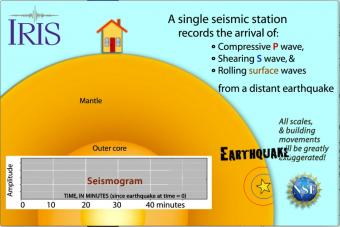
Seismic waves travel through the earth to a single seismic station. Scale and movement of the seismic station are greatly exaggerated to depict the relative motion recorded by the seismogram as P, S, and surface waves arrive.
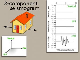
We use exaggerated motion of a building (seismic station) to show how the ground moves during an earthquake, and why it is important to measure seismic waves using 3 components: vertical, N-S, and E-W. Before showing an actual distant earthquake, we break down the three axes of movement to clarify the 3 seismograms.
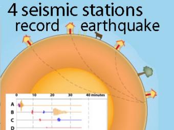
A cow and a tree in this narrated cartoon for fun and to emphasize that seismic waves traveling away from an earthquake occur everywhere, not just at seismic stations A, B, C, and D. A person would feel a large earthquake only at station A near the epicenter. Stations B, C, D, and the cow are too far from the earthquake to feel the seismic waves though sensitive equipment records their arrival.
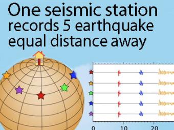
A gridded sphere is used to show a single station recording five equidistant earthquakes.
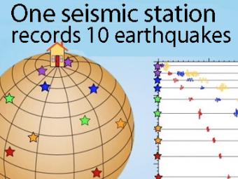
A gridded sphere is used to show: 1) the seismic stations don't need to be lined up longitudinally to create travel-time curves, as they appear in the first animation, and 2) a single station records widely separated earthquakes that plot on the travel-time curves.
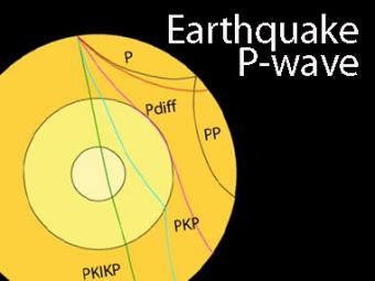
The shadow zone is the area of the earth from angular distances of 104 to 140 degrees from a given earthquake that does not receive any direct P waves. The different phases show how the initial P wave changes when encountering boundaries in the Earth.
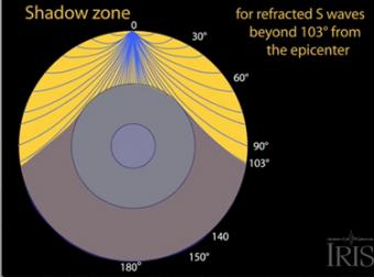
The shadow zone results from S waves being stopped entirely by the liquid core. Three different S-wave phases show how the initial S wave is stopped (damped), or how it changes when encountering boundaries in the Earth.
Related Fact-Sheets
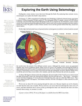
Earthquakes create seismic waves that travel through the Earth. By analyzing these seismic waves, seismologists can explore the Earth's deep interior. This fact sheet uses data from the 1994 magnitude 6.9 earthquake near Northridge, California to illustrate both this process and Earth's interior structure.
NOTE: Out of Stock; self-printing only.
Related Software-Web-Apps
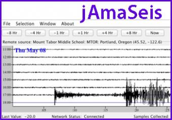
jAmaSeis is a free, java-based program that allows users to obtain and display seismic data in real-time from either a local instrument or from remote stations.
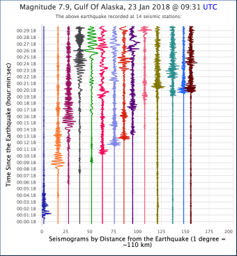
Seismic Waves is a browser-based tool to visualize the propagation of seismic waves from historic earthquakes through Earth’s interior and around its surface. Easy-to-use controls speed-up, slow-down, or reverse the wave propagation. By carefully examining these seismic wave fronts and their propagation, the Seismic Waves tool illustrates how earthquakes can provide evidence that allows us to infer Earth’s interior structure.
Related Videos
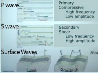
Video lecture on wave propagation and speeds of three fundamental kinds of seismic waves.
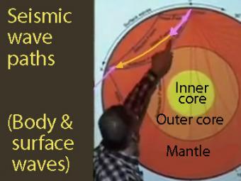
A video demonstration of how a slinky can be a good model for illustrating P & S seismic waves movement.
Related Lessons
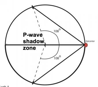
Students work first in small groups, and then as a whole class to compare predicted seismic wave travel times, generated by students from a scaled Earth model, to observed seismic data from a recent earthquakes. This activity uses models, real data and emphasizes the process of science.
To understand plate tectonic processes and hazards, and to better understand where future earthquakes are likely to occur, it is important to locate earthquakes as they occur. In this activity students use three-component seismic data from recent earthquakes to locate a global earthquake.
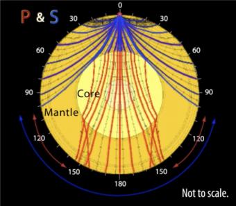
In this multi-step lab, students explore the concepts of seismic wave propagation through materials with different mechanical properties, and examine seismic evidence from a recent earthquake to infer Earth’s internal structure and composition. This lab is designed to be done with an instructor present to answer questions and guide students to conclusions
Related Posters
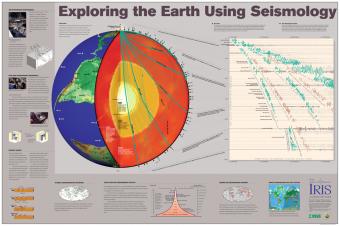
Seismic waves from earthquakes ricochet throughout Earth's interior and are recorded at geophysical observatories around the world. The paths of some of those seismic waves and the ground motion that they caused are used by seismologists to illuminate Earth's deep interior.
We encourage the reuse and dissemination of the material on this site as long as attribution is retained. To this end the material on this site, unless otherwise noted, is offered under Creative Commons Attribution ( CC BY 4.0 ) license
- Mailing Lists
- Frequently Asked Questions
- Privacy Policy
- Terms of Service
- Comments about this page
- Instrumentation Services
- Data Services


IMAGES
COMMENTS
Jump to. A travel graph is a line graph which describes a journey - it shows how distance changes with time. Time is always represented on the x-axis and distance on the y-axis. The distance is ...
The distance travelled is the area under the graph. The acceleration and deceleration can be found by finding the gradient of the lines. On travel graphs, time always goes on the horizontal axis (because it is the independent variable). Trapezium Rule. This is a useful method of estimating the area under a graph.
To make things easier, we can separate this graph into shapes: 2 triangles and 1 rectangle. Triangle 1: Area of a triangle = ½ × base of triangle × height of triangle. Area = ½ × 4 km × 3 km/min. Area = 6 km2. Rectangle: Length of the rectangle can be found by finding out the difference between 50 and 4, which equals to 46 min. The height ...
Travel graphs are line graphs that are used to describe the motion of objects such as cars, trains, walkers and cyclists. The distance travelled is represented on the vertical axis and the time taken to travel that distance is represented on the horizontal axis. The following graph gives the distance of a cyclist from his home. a.
More resources available at www.misterwootube.com
Travel graphs are a way to describe the movement of people or objects. They usually describe a trip that leaves and returns to a point (like a home base). The vertical axis of a travel graph is the distance travelled from a starting point and the horizontal axis is the time taken from the starting point. Reading a travel graph
Level 4 - Draw a travel graph from the given description. Exam Style Questions - A collection of problems in the style of GCSE or IB/A-level exam paper questions (worked solutions are available for Transum subscribers). More Graphs including lesson Starters, visual aids, investigations and self-marking exercises.
Choose a scale to represent the distance and another to represent the time on the graph. For the motion of the car scales could be Time: 1 min = 1 cm and Distance: 1 km = 1 cm. Mark values for the time and the distance on the respective axes. Now you have to mark the points on the graph paper to represent each set of values for distance and time.
In this educational video, we dive into the fascinating world of travel graphs. Join us as we explore the concepts of acceleration, distance, and speed, and ...
Learn better and improve your grades. Find more lesson videos like this and learn more about mathematics in the Prime Learn App.👉Visit us at - http://www.pr...
Reading travel graphs. A travel graph shows the distance travelled away from a set point against the time. This allows us to identify the speed at which they have travelled, points at which they ...
Travel Graphs GCSE Revision Description. This set of questions provides travel graphs in the form of distance-time graphs. Learners will need to read information from the graphs, such as distances at certain times and periods of rest. They will also need to calculate the speed between different times.
GCSE Maths: Travel Graphs (Speed-Distance-Time) Watch on. This is the second lesson in a new series with the Maths Appeal duo - Bobby Seagull and Susan Okereke - and Tom Rocks Maths where we'll be exploring the GCSE Maths syllabus to show the world that maths is accessible to everyone! Watch Bobby and Susan answer YOUR questions here.
In this lesson, we will interpret distance-time graphs. We will answer questions regarding how far or how long a journey has been at different points, segments, and overall. This quiz includes images that don't have any alt text - please contact your teacher who should be able to help you with an audio description.
This is level 4; Draw a travel graph from the given description. Click on the points at the ends of where the straight line segments of the graphs should be. Cycling to work. Draw a distance-time graph show the journey a computer programmer makes by bicycle to work each day. The distance from home to work is eight kilometres and she has to stop ...
Level 4 - Draw a travel graph from the given description. Exam Style Questions - A collection of problems in the style of GCSE or IB/A-level exam paper questions (worked solutions are available for Transum subscribers). More Graphs including lesson Starters, visual aids, investigations and self-marking exercises.
Learn how to use travel graphs relating speed, distance and time to solve problems. Tom introduces the topic, Bobby applies it to Usain Bolt's 100-metre worl...
(b) Explain how you can tell from the graph that it took less time to travel the first 70km of the journey than it took to travel the final 70km of the journey. The distance-time graph shows a 140km journey from Meadow Green to Tarn Close. Distance in km Tarn Close 140 120 100 Time Meadow Green O 12:00 13:00 14:00 15:00 (a) (i) (ii) 16:00
How do I draw an acceleration-time graph? Most of the time the acceleration will be constant so you have to draw horizontal lines; There will be discontinuities in the graph if the object instantaneously changes from acceleration at a constant rate to moving with constant velocity; The area between an acceleration-time graph and the x-axis is the change in velocity
In Y8, you covered distance-time graphs and this year we will move on to velocity-time graphs. Although the graphs of a distance-time and a velocity-time graph may be equal, they describe very different journeys, as shown by the starter. E.g.1 The gradient of a distance-time graph is the rate of change of distance with respect to time
Description of activity. For each of the six travel graphs, students will be asked to write a brief description of the journey that the graph might represent. Students will complete the accompanying worksheet. Context. Patterns and Algebra, Working Mathematically.
Select the cheapest unused edge in the graph. 2. Repeat step 1, adding the cheapest unused edge to the circuit, unless: a. adding the edge would create a circuit that doesn't contain all vertices, or. b. adding the edge would give a vertex degree 3. 3. Repeat until a circuit containing all vertices is formed.
Travel Graphs - irp-cdn.multiscreensite.com
A travel time curve is a graph of the time that it takes for seismic waves to travel from the epicenter of an earthquake to seismograph stations at varying distances away. The velocity of seismic waves through different materials yield information about Earth's deep interior. IRIS' travel times graphic for the 1994 Northridge, CA earthquake ...