travelling salesman math ia

Plus.Maths.org

The travelling salesman

On 20th November 2012 Plus hosted the first UK screening of Travelling Salesman , an intellectual thriller imagining the consequences of solving the P vs NP problem, at the Centre for Mathematical Sciences in Cambridge. Here you can find out what this problem is all about.

We're hosting another screening of the film on 14 March 2013, Pi Day, as part of the Cambridge Science Festival

Get cash from the cash point, go to the supermarket, pick up kids from school and prescription from doctor. In what order should you do these things so that the distance you've got to drive is as short as possible? Not a particularly exciting problem, you might think, but it's one that fascinates mathematicians. That's because in general it's very hard to solve and opens the door on one of the trickiest unanswered questions in mathematics.

The problem is called the travelling salesman problem and the general form goes like this: you've got a number of places to visit, you're given the distances between them, and you have to work out the shortest route that visits every place exactly once and returns to where you started. If it's a small number of places, you can find the answer quite easily simply by looking at all the possible routes. As the number of places grows, this becomes incredibly tedious. Is there a better method for doing this, an algorithm, that can give you an answer in a reasonable amount of time even if the number of places is huge?

The functions 2 n (black), n 3 (red) and n 2 plotted against n. You can see that 2 n grows fastest for larger n.

The collection of all decision problems for which a possible answer can be verified easily (in the sense that there’s a polynomial-time algorithms for checking the answer) has a name: it’s called the NP class. Another problem in that class is how to factorise large numbers into primes, for example working out that

Once you know the prime factors of a number it’s easy to check that they are correct, you only need to multiply, but nobody knows of any polynomial-time algorithms to find these factors in the first place.

This leads us to the big question: are there any polynomial-time algorithms for problems in the NP class that simply haven't been discovered yet? The question is known as the P versus NP problem because the class of problems that can be solved in polynomial time is called P. P versus NP is one of the hardest open problems in maths. Anyone who manages to answer it will win $1 million from the Clay Mathematics Institute (see How maths can make you rich and famous ). Not everyone agrees, but most mathematicians seem to think that P is not equal to NP: this would mean that NP problems really are very difficult, they cannot be solved in polynomial time.

Answers to NP problems can be used as the key to encrypted messages.

And there's another twist to the story: any problem in the NP class can actually be reduced to the decision version of the travelling salesman problem. This means that any algorithm that solves the decision travelling salesman problem can be translated into one that solves all other problems in the NP class. So imagine you find a polynomial-time algorithm for the decision travelling salesman problem. This would then mean that every problem in NP could be solved in polynomial time, you would have proved that P=NP and could go and collect your $1 million. (And the same would be true if you found such an algorithm for the harder, general version of the travelling salesman problem.)

But there are other implications too. Problems from the NP class are often used in cryptography, for example in the RSA system that's used to make internet transactions secure. Essentially, the answer to an NP problem (say the prime factors of a large number) is used as the key you need to decode a message. The fact that there are no known algorithms to solve NP problems quickly means that the key is very hard to crack. (See Safety in numbers for more.)

So imagine you did manage to find an efficient algorithm to solve the travelling salesman problem. You'd get your million dollars, a key to the world's most secret codes and your life would probably no longer be safe. Someone should make a movie about this...

• Add new comment

A new 'Shrink' algorythm resolves the TSP problem at a rate of n^3*7E-5 secs. 100 nodes take 2 seconds on a 1.8Ghz PC running on a QPC2 emulator with a procedural basic. Timings were done by a Professor of mathematics at Delaware State university. The code can surely be optimised, and produces a 94% accurate result as things stand, but this will be improved on. The maths are very simple, but the logic is quite complex. The program was published by the English 'Quanta' QL users group, and is available for programmers to work on.

The travelling salesman problem

TSP solved? I am not sure! I believe tha I have found the effective algoritm for the shortest route to take. I have contacted The Clay Mathematics Institute for how to present my solution. Sincerely, Dr Lars Hellström, Uppsala, Sweden

Travelling caregiver problem

Real world gets more complicated than the salesman pitch.

In the real world, the factors influencing the optimal outcome: * is it faster to do tasks without kids (or persons cared for), * how much time do you have to complete all tasks, * is it cheaper to be quick, or take shortest route?

I have no algorithm but these factors affect my decision-making every day to maximise my 24 hours.

Traveling Caregiver Problem

1. "Mum" has scientifically reduced the problem to its essence. Never take the kids to the grocery store if efficiency is your first concern. So go there first. 2. Solve as much of the problem once and for all in advance as possible. Never go to an ATM (if that's what a pay point is). Get a Paypal account, move cash into it online, and use the Paypal card instead of cash. Easier, more secure, eliminates one stop on the trip, and gives you a record of what you spent and where, making budgeting simpler (thus reducing another set of math and tracking problems). 3. Change your prescriptions to three-month refills or better, delivered by mail. There -- two trips out of three to the pharmacy, or all of them, eliminated. 4. The Law of Scientific Parsimony absolutely dictates: Never give a problem to a mathematician if a Mum can solve it. This approach has been proven by experience to work for up to whatever number of children are in your family.

And if you really need to pretend this is a math/geography problem: It is not. It's a management question. The first parameter to plug in is the likelihood of the traveling salesman closing a deal, and how big, at each destination. Send him to the likeliest big deals first and hit the marginal ones up with a phone call. Be very wary of trying to apply math to social-interaction questions with small sample sizes.

Glad to be of assistance.

Programming Assignment Help

I really appreciate your effort in providing this kind of content to us.

Agreed - avoid it if possible

"Mum" has it spot on, as usual. I teach advanced server performance tuning, and the first thing I ask new students is "what's the fastest way to get from London to Glasgow ?" (I live in UK). Answer: don't go to Glasgow, have a video call instead. In IT you can't make the hardware go faster (e.g. if a disk spins round at 10,000rpm, that's what it does, no amount of blowing on it will make it spin round faster) so the only way to "speed up" disk IOs is … you can't. You have to eliminate some of them. Just like Mum's Paypal account.

TSP Solution

Don't tell me...you just couldn't fit the answer in comment box?

Traveling Salesman Problem

The Traveling Salesman Problem, or TSP for short, is one of the most intensively studied problems in computational mathematics. These pages are devoted to the history, applications, and current research of this challenge of finding the shortest route visiting each member of a collection of locations and returning to your starting point.

The work described here is supported by the Natural Sciences and Engineering Research Council of Canada (NSERC) and the Department of Combinatorics and Optimization at the University of Waterloo .

IB DP Maths Topic 10.10 Travelling salesman problem. HL Paper 3

IB DP Physics IB DP Maths IB DP Chemistry IB DP Biology

  Download IITian Academy  App for accessing Online Mock Tests and More..

A graph G with vertices A, B, C, D, E has the following cost adjacency table.

\[\begin{array}{*{20}{c|ccccc}}   {}&{\text{A}}&{\text{B}}&{\text{C}}&{\text{D}}&{\text{E}} \\ \hline   {\text{A}}& – &{12}&{10}&{17}&{19} \\   {\text{B}}&{12}& – &{13}&{20}&{11} \\   {\text{C}}&{10}&{13}& – &{16}&{14} \\   {\text{D}}&{17}&{20}&{16}& – &{15} \\   {\text{E}}&{19}&{11}&{14}&{15}& –   \end{array}\]

(a)     (i)     Use Kruskal’s algorithm to find and draw the minimum spanning tree for G .

  (ii)     The graph H is formed from G by removing the vertex D and all the edges connected to D. Draw the minimum spanning tree for H and use it to find a lower bound for the travelling salesman problem for G .

(b)     Show that 80 is an upper bound for this travelling salesman problem.

(a)     (i)     the edges are joined in the order

Note: Final A1 independent of the previous A2 .

the weight of this spanning tree is 33     A1

to find a lower bound for the travelling salesman problem, we add to that the two smallest weights of edges to D, i.e. 15 +16, giving 64     M1A1

(b)     an upper bound is the weight of any Hamiltonian cycle, e.g. ABCDEA has weight 75 so 80 is certainly an upper bound     M1A1

Total [9 marks]

Examiners report

Part (a) was well done by many candidates although some candidates simply drew the minimum spanning tree in (i) without indicating the use of Kruskal’s Algorithm. It is important to stress to candidates that, as indicated in the rubric at the top of Page 2, answers must be supported by working and/or explanations. Part (b) caused problems for some candidates who obtained the unhelpful upper bound of 96 by doubling the weight of the minimum spanning tree. It is useful to note that the weight of any Hamiltonian cycle is an upper bound and in this case it was fairly easy to find such a cycle with weight less than or equal to 80.

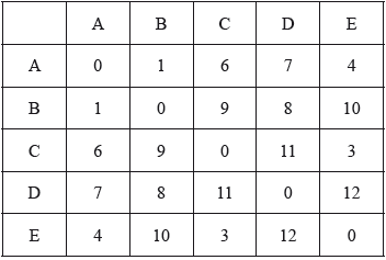
The complete graph H has the following cost adjacency matrix.

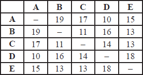
Consider the travelling salesman problem for H .

a.By first finding a minimum spanning tree on the subgraph of H formed by deleting vertex A and all edges connected to A, find a lower bound for this problem. [5]

b.Find the total weight of the cycle ADCBEA. [1]

c.What do you conclude from your results? [1]

using any method, the minimum spanning tree is     (M1)

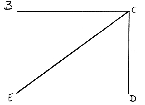
Note: Accept MST = {BC, EC, DC} or {BC, EB, DC}

Note: In graph, line CE may be replaced by BE.

lower bound = weight of minimum spanning tree + 2 smallest weights connected to A     (M1)

= 11 + 13 + 14 + 10 + 15 = 63     A1

weight of ADCBEA = 10 + 14 + 11 + 13 + 15 = 63     A1

the conclusion is that ADCBEA gives a solution to the travelling salesman problem     A1

This question was generally well answered although some candidates failed to realise the significance of the equality of the upper and lower bounds.

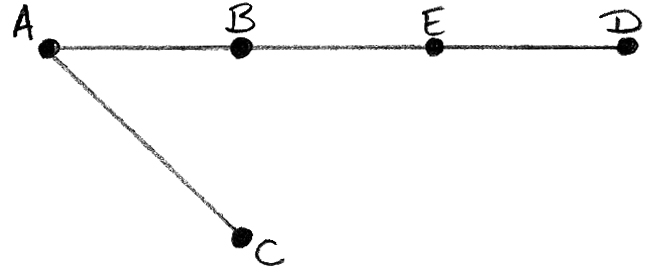
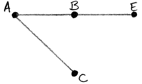
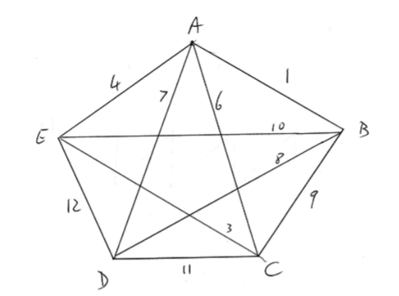
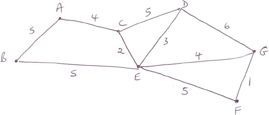
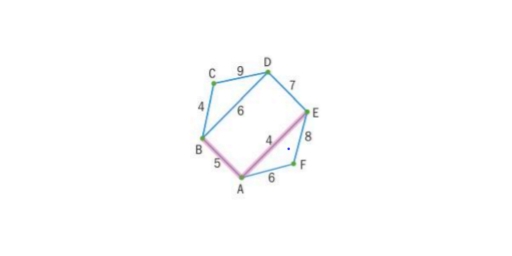
The following diagram shows a weighted graph G with vertices A, B, C, D and E.

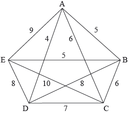
a.Show that graph \(G\) is Hamiltonian. Find the total number of Hamiltonian cycles in \(G\), giving reasons for your answer. [3]

b.State an upper bound for the travelling salesman problem for graph \(G\). [1]

d.Hence find a lower bound for the travelling salesman problem for \(G\). [2]

e.Show that the lower bound found in (d) cannot be the length of an optimal solution for the travelling salesman problem for the graph \(G\). [3]

eg the cycle \({\text{A}} \to {\text{B}} \to {\text{C}} \to {\text{D}} \to {\text{E}} \to {\text{A}}\) is Hamiltonian     A1

starting from any vertex there are four choices

from the next vertex there are three choices, etc …     R1

so the number of Hamiltonian cycles is \(4!{\text{ }}( = 24)\)     A1

Note: Allow 12 distinct cycles (direction not considered) or 60 (if different starting points count as distinct). In any case, just award the second A1 if R1 is awarded.

total weight of any Hamiltonian cycles stated

eg \({\text{A}} \to {\text{B}} \to {\text{C}} \to {\text{D}} \to {\text{E}} \to {\text{A}}\) has weight \(5 + 6 + 7 + 8 + 9 = 35\)     A1

a lower bound for the travelling salesman problem is then obtained by adding the weights of CA and CB to the weight of the minimum spanning tree     (M1)

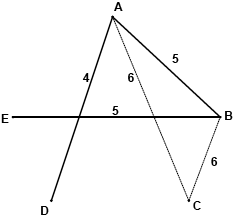
a lower bound is then \(14 + 6 + 6 = 26\)     A1

eg eliminating A from G, a minimum spanning tree of weight 18 is     (M1)

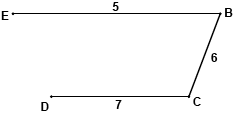
adding AD and AB to the spanning tree gives a lower bound of \(18 + 4 + 5 = 27 > 26\)     A1

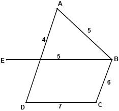
so 26 is not the best lower bound     AG

Note:  Candidates may delete other vertices and the lower bounds obtained are B-28, D-27 and E-28.

there are 12 distinct cycles (ignoring direction) with the following lengths

Cycle     Length

ABCDEA     35     M1

ABCEDA     33

ABDCEA     39

ABDECA     37

ABECDA     31

ABEDCA     31

ACBDEA     37

ACBEDA     29

ACDBEA     35

ACEBDA     33

AEBCDA     31

AECBDA     37     A1

as the optimal solution has length 29     A1

26 is not the best possible lower bound     AG

Note:  Allow answers where candidates list the 24 cycles obtained by allowing both directions.

Part (a) was generally well answered, with a variety of interpretations accepted.

Part (b) also had a number of acceptable possibilities.

Part (d) was generally well answered, but there were few good attempts at part (e).

The weighted graph K , representing the travelling costs between five customers, has the following adjacency table.

a.Draw the graph \(K\). [2]

b.Starting from customer D, use the nearest-neighbour algorithm, to determine an upper bound to the travelling salesman problem for K . [4]

c.By removing customer A, use the method of vertex deletion, to determine a lower bound to the travelling salesman problem for K . [4]

complete graph on five vertices     A1

weights correctly marked on graph     A1

clear indication that the nearest-neighbour algorithm has been applied     M1

DA (or 7)     A1

AB (or 1) BC (or 9)     A1

CE (or 3), ED (or 12), giving UB = 32     A1

attempt to use the vertex deletion method     M1

minimum spanning tree is ECBD     A1

(EC 3, BD 8, BC 9 total 20)

reconnect A with the two edges of least weight, namely AB (1) and AE (4)     M1

lower bound is 25     A1

a.The weights of the edges of a graph \(H\) are given in the following table.

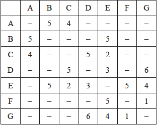
(i)     Draw the weighted graph \(H\).

(ii)     Use Kruskal’s algorithm to find the minimum spanning tree of \(H\). Your solution should indicate the order in which the edges are added.

(iii)     State the weight of the minimum spanning tree. [8]

b.Consider the following weighted graph.

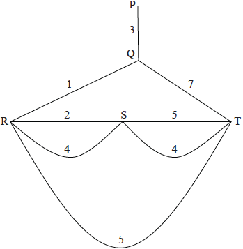
(i) Write down a solution to the Chinese postman problem for this graph.

(ii) Calculate the total weight of the solution. [3]

c.(i)     State the travelling salesman problem.

(ii)     Explain why there is no solution to the travelling salesman problem for this graph. [3]

Note:     Award A1 if one edge is missing. Award A1 if the edge weights are not labelled.

(ii)     the edges are added in the order:

\(FG{\rm{ }}1\)     M1A1

\(CE{\rm{ }}2\)      A1

\(ED{\rm{ }}3\)

\(EG{\rm{ }}4\)      A1

\(AC{\rm{ }}4\)

Note:      \(EG\) and  \(AC\) can be added in either order.

(Reject \(EF\) )

(Reject \(CD\) )

\(EB5\) OR  \(AB5\)     A1

Notes:     The minimum spanning tree does not have to be seen.

If only a tree is seen, the order by which edges are added must be clearly indicated.

(iii)      \(19\)     A1

(i)     eg ,  \(PQRSRTSTQP\) OR  \(PQTSTRSRQP\)     M1A1

Note:     Award M1 if in either (i) or (ii), it is recognised that edge  \(PQ\) is needed twice.

(ii)     total weight \( = 34\)     A1

(i)     to determine a cycle where each vertex is visited once only (Hamiltonian cycle)     A1

of least total weight     A1

(ii)     EITHER

to reach \(P\), \(Q\) must be visited twice which contradicts the definition of the \(TSP\)     R1

the graph is not a complete graph and hence there is no solution to the \(TSP\)     R1

Total [14 marks]

Part (a) was generally very well answered. Most candidates were able to correctly sketch the graph of \(H\) and apply Kruskal’s algorithm to determine the minimum spanning tree of \(H\). A few candidates used Prim’s algorithm (which is no longer part of the syllabus).

Most candidates understood the Chinese Postman Problem in part (b) and knew to add the weight of \(PQ\) to the total weight of \(H\). Some candidates, however, did not specify a solution to the Chinese Postman Problem while other candidates missed the fact that a return to the initial vertex is required.

In part (c), many candidates had trouble succinctly stating the Travelling Salesman Problem. Many candidates used an ‘edge’ argument rather than simply stating that the Travelling Salesman Problem could not be solved because to reach vertex \(P\), vertex \(Q\) had to be visited twice.

Wolfram|Alpha Widgets Overview Tour Gallery Sign In

Share this page.

• StumbleUpon
• Google Buzz

Output Type

Output width, output height.

To embed this widget in a post, install the Wolfram|Alpha Widget Shortcode Plugin and copy and paste the shortcode above into the HTML source.

To embed a widget in your blog's sidebar, install the Wolfram|Alpha Widget Sidebar Plugin , and copy and paste the Widget ID below into the "id" field:

Save to My Widgets

Build a new widget.

We appreciate your interest in Wolfram|Alpha and will be in touch soon.

• Speakers & Mentors
• AI services

Solving Notorious Traveling Salesman with Cutting-Edge AI Algorithms

Solving the notorious traveling salesman problem with cutting-edge ai.

The traveling salesman problem (TSP) is arguably one of the most iconic and challenging combinatorial optimization problems in computer science and operations research. At its core, this notorious NP-hard problem deals with finding the shortest route visiting each city in a given list exactly once, before returning to the starting city.

Despite its simple formulation, TSP exemplifies an optimization problem that quickly grows to staggering complexity as the number of cities increases. Its difficulty stems from the factorial growth of possible routes to evaluate with added cities. And to make matters worse, TSP belongs to a special class of the most difficult problems with no known efficient solution – it is NP-hard.

Yet, the traveling salesman problem and its numerous variants continuously captivate researchers. The practical applications of TSP span far and wide, including vehicle routing, tool path optimization, genome sequencing and a multitude of logistics operations. It comes as no surprise that intense efforts have been devoted to developing efficient methods for obtaining high-quality solutions.

In recent years, AI has opened new possibilities for tackling TSP. Modern techniques powered by neural networks and reinforcement learning hold promise to push the boundaries. This article reviews the advances of AI for solving the traveling salesman conundrum. We dive into the capabilities of leading approaches, hybrid methods, innovations with deep learning and beyond.

The Allure of the Traveling Salesman

The origins of TSP date back centuries, with the general premise being discussed in the 1800s. Mathematicians like W.R. Hamilton and Thomas Kirkman proposed early mathematical formulations of the problem during that era. But it was not until the 1930s that the general form was rigorously studied by Karl Menger and others at Harvard and Vienna.

The standard version of TSP entered mainstream research in the 1950s and 1960s. Mathematicians Hassler Whitney and Merrill Flood at Princeton University promoted the problem within academic circles. In a landmark paper published in 1956, Flood described heuristic methods like nearest neighbor and 2-opt for generating good feasible tours.

As computer technology advanced in the 1950s, scientists were able to test algorithms on progressively larger problem instances. But even the fastest computers could not escape the exponential growth in the search space. Out of curiosity, what would be the approximate number of possible routes for a 100-city tour? It is estimated at 10^155, an astronomically large number exceeding the number of atoms in the universe!

The traveling salesman problem has become a workhorse for testing optimization algorithms. TSP exemplifies the challenges of combinatorial optimization in a nutshell. It serves as a standard benchmark to evaluate new algorithms. As well, techniques developed for TSP often provide inspiration to address other hard optimization problems.

Exact Algorithms: Success Limited by Complexity

The most straightforward approach for TSP is to systematically enumerate all tours, then select the one with minimum distance. This trivial algorithm guarantees the optimal solution. But it quickly becomes intractable as the number of cities grows, due to the exponential explosion of possible tours. Even fast modern computers cannot get far with brute-force enumeration.

More sophisticated algorithms use intelligent pruning rules to avoid evaluating unnecessary tours. These exact algorithms can prove optimality, but remain limited by combinatorial complexity.

A prominent example is Held and Karp’s branch-and-bound algorithm published in 1962. It systematically constructs a search tree, branching on each city pair to start a sub-tour. Bounding rules prune branches with cost exceeding the best solution found so far. With careful implementation, the Held-Karp algorithm can optimally solve instances up to about 25 cities.

Further improvements have been made over the decades, such as integrating cutting planes and other methods to tighten bounds. Exact algorithms have managed to push the limits, optimally solving TSPs with tens of thousands of cities in some cases. But beyond a certain scale, the exponential growth renders complete enumeration utterly hopeless.

Heuristics and Local Search: Near-Optimal Solutions

For larger instances of TSP, heuristics that efficiently find good feasible solutions become essential. Local search heuristics iteratively improve an initial tour by making beneficial modifications guided by cost gradients. Well-designed heuristics can routinely find tours within a few percent of optimal.

The nearest neighbor algorithm provides a simple constructive heuristic to build a tour incrementally. It starts from a random city, repeatedly visiting the closest unvisited city until all have been added. Despite its greediness, nearest neighbor quickly yields short tours.

Local search heuristics start from a tour, then explore neighbor solutions iteratively. Moves that reduce the tour length are accepted, allowing “downhill” descent toward better tours. Variants of the 2-opt algorithm are widely used, where two edges are replaced by two alternative edges to form a neighbor solution.

More advanced heuristics like Lin-Kernighan also allow occasional uphill moves to escape local optima. Modern implementations can fine-tune routes using complex rules and heuristics specialized for TSP. While not guaranteed to find optimal tours, well-tuned local search algorithms regularly find solutions less than 1% away from optimal.

Approximation Algorithms: Guaranteed Worst-Case Performance

Approximation algorithms provide a tour along with a guarantee that the length is within a certain factor of optimal. These algorithms assure a solution quality on any problem instance, in contrast to heuristics tailored and tuned for typical instances.

A simple approximation algorithm stems from a minimum spanning tree solution. By visiting cities according to a minimum spanning tree order, then taking shortest paths between each, one obtains a tour costing no more than twice optimal. This easy 2-approximation solution admits a worst-case optimality proof.

More sophisticated algorithms like Christofides provide a 1.5-approximation for TSP. Extensions incorporating machine learning have shown empirical improvements while maintaining theoretical approximation guarantees. The best known approximation factor for TSP currently stands at 1.299 using an algorithm by Anari and Oveis Gharan.

Evolutionary Algorithms: Optimization by Natural Selection

Evolutionary algorithms take inspiration from biological principles of mutation, recombination and natural selection. Candidate solutions represent individuals in a population. The fitness of each depends on the tour length, where shorter tours yield higher fitness. In each generation, high fitness individuals are probabilistically chosen to reproduce via recombination and mutation operators. The population evolves toward fitter solutions over successive generations via this artificial selection.

Genetic algorithms are a popular class of evolutionary technique applied to TSP. Other variants exist, including memetic algorithms that hybridize evolutionary search with local optimization. Evolutionary methods can provide high-quality solutions when properly tuned. They intrinsically perform a broad exploration of the search space, less prone to stagnation in local optima compared to local search.

Neural Networks: Learning to Construct Tours

Artificial neural networks provide state-of-the-art tools to automate algorithm design. Neural approaches for TSP take advantage of modern deep learning, training networks to produce high-quality tours via exposure to problem examples.

Recall that the search space for TSP grows factorially with cities. But optimal solutions tend to share intuitive patterns, like visiting clusters of nearby cities consecutively. Neural networks are well suited to automatically extract such latent patterns by generalizing from examples. This facilitates efficient construction of new tours sharing properties of high-performing ones.

Specific neural architectures for TSP include graph convolutional neural networks, self-organizing maps, attention-based seq2seq models, and reinforcement learning. Next we highlight a few leading neural approaches.

Graph Neural Networks

Graph convolutional neural networks (GCNNs) operate directly on graph representations of TSP instances. The networks embed graph structure into a neural feature space. Learned features help inform graph algorithms to construct tours reflecting patterns underlying high-quality solutions.

GCNNs have shown promising results, achieving near state-of-the-art performance on TSPs up to 100 cities. Extensions augment neural features with heuristic algorithms like 2-opt to further boost performance.

Attention-Based Sequence-to-Sequence

Casting TSP as a set-to-sequence problem has enabled application of seq2seq neural architectures. The set of city nodes is fed into an encoder network that produces a contextual feature representation. Attention-based decoding sequentially outputs a tour by predicting the next city at each step.

Notably, the Transformer architecture (popularized for language tasks) has been adapted for TSP. The self-attention mechanism helps model complex interactions when determining the incremental tour construction. Empirical results on TSPs with up to 100 nodes are competitive with other neural methods.

Reinforcement Learning

Reinforcement learning (RL) provides a natural framework for solving sequential decision problems like TSP. The decisions correspond to selecting the next city to extend the tour under construction. Reward signals relate to tour cost. By optimizing policies maximizing long-term reward, RL agents learn heuristics mimicking high-quality solutions.

Actor-critic algorithms that combine policy gradient optimization with value function learning have been applied successfully. Graph embedding networks help leverage problem structure. RL achieves strong empirical performance on 2D Euclidean TSP benchmarks. Ongoing research extends RL capabilities to larger graphs.

Hybrid Methods: Combining Strengths

Hybrid techniques aim to synergistically blend components such as machine learning, combinatorial algorithms, constraint programming, and search. TSP provides an ideal testbed for hybrids given its long history and extensive algorithmic literature.

One approach trains graph neural networks to predict edge costs relating to inclusion regret. These guide local search algorithms like 2-opt or Lin-Kernighan over transformed edge weights. The hybrid model achieves state-of-the-art results by interleaving learning-based preprocessing and classic iterative improvement.

Other work combines evolutionary algorithms with deep reinforcement learning. Evolutionary search provides broad exploration while neural networks exploit promising regions. Such hybrids demonstrate improved robustness and scalability on challenging TSP variants with complex side constraints.

Ongoing initiatives explore orchestrating machine learning, global search and solvers dynamically. Early experiments optimizing collaboration strategies show promise on difficult TSP instances. Intelligently integrated hybrids are poised to push boundaries further.

Innovations and Open Problems

While much progress has been made applying AI to TSP, challenges remain. Developing algorithms that scale effectively to problems with thousands of cities or complex side constraints is an active research direction. Expanding capabilities to handle diverse graph structures beyond Euclidean instances poses difficulties. Optimizing the interplay between learning and search in hybrid methods has ample room for innovation.

Open questions remain about how to design neural architectures that fully capture the structure and complexity underlying rich TSP variants. Dynamic and stochastic TSP scenarios require extending neural models to handle time, uncertainty and risk considerations. While deep reinforcement learning has shown promise on small instances, scaling up efficiently remains an open problem.

As algorithmic advances enable solving larger TSPs close to optimality, the boundaries of problem complexity will be tested. Scientists also continue developing new theoretically grounded algorithms with guaranteed solution quality. Further innovations in AI and hybrid techniques will push forward the state of the art on this captivating optimization challenge.

The traveling salesman problem has become an optimization icon after decades of intensive study. While TSP is easy to state, locating optimal tours rapidly becomes intractable as the number of cities grows. Exact algorithms can prove optimality for problems up to a few thousand cities. Very large instances with millions of cities remain out of reach.

For practical applications, near-optimal solutions are often sufficient. Heuristics and local search algorithms capably handle large TSPs with thousands of cities. Well-tuned heuristics routinely find tours within 1-2% of optimal using fast local improvement rules.

Modern AI brings fresh ideas to advance TSP algorithms. Neural networks show impressive performance by generalizing patterns from training examples. Deep reinforcement learning adapts solutions through trial-and-error experience. Hybrid techniques synergistically integrate machine learning with algorithms and search.

Yet many fascinating challenges remain. Developing AI methods that scale effectively to massive problem sizes and complex variants poses research frontiers. Integrating global exploration with intensive local refinement is key for difficult instances. Advances in hybrid algorithms also rely on optimizingdynamic collaboration between learning modules.

The traveling salesman journey continues as innovators build on past work to propel solution quality forward. AI opens new horizons to rethink how optimization algorithms are designed. As researchers traverse new ground, undoubtedly the notorious TSP has much more in store on the road ahead!

Comparing Leading AI Approaches for the Traveling Salesman Problem

Artificial intelligence offers a versatile collection of modern techniques to address the traveling salesman problem. The core challenge involves finding the shortest tour visiting each city exactly once before returning to start. This famous NP-hard problem has captivated researchers for decades, serving as a platform to test optimization algorithms.

In recent years, AI has opened new possibilities for tackling TSP. Cutting-edge methods powered by machine learning achieve impressive performance by learning from examples. This article provides an in-depth comparison of leading AI approaches applied to the traveling salesman problem.

We focus the analysis on four prominent categories of techniques:

• Graph neural networks
• Reinforcement learning
• Evolutionary algorithms
• Hybrid methods

By reviewing the problem-solving process, capabilities and limitations, we gain insight into how algorithmic innovations impact solution quality. Understanding relative strengths and weaknesses helps guide future progress.

How Algorithms Approach Solving TSP

The high-level search process differs substantially across AI methods:

Graph neural networks learn structural patterns from training instances with optimal/near-optimal tours. Learned features help construct new tours reflecting examples.

Reinforcement learning incrementally extends tours, relying on reward feedback to improve the construction policy. Trial-and-error experience shapes effective heuristics.

Evolutionary algorithms maintain a population of tours, iteratively selecting fit individuals to reproduce via crossover and mutation. The population evolves toward higher quality solutions.

Hybrid methods orchestrate components like machine learning, combinatorial heuristics and search. Collaboration strategies are optimized to benefit from complementary capabilities.

These differences influence their optimization trajectories and performance profiles. Next we dive deeper into solution quality, scalability, speed and limitations.

Solution Quality

Graph neural networks achieve strong results by generalizing patterns, reaching near state-of-the-art performance on moderate TSP sizes. Attention mechanisms help capture dependencies when constructing tours.

Reinforcement learning develops high-performing policies through repeated practice. RL matches or exceeds human-designed heuristics, excelling on 2D Euclidean TSPs. Challenging instances with complex constraints remain difficult.

Evolutionary algorithms effectively explore the solution space and find near-optimal tours when well-tuned. Recombination of parental solutions provides beneficial genetic variation. Performance depends heavily on hyper-parameters and operators.

Hybrid methods produce state-of-the-art results by orchestrating components intelligently. Learning-based preprocessing guides local search, while global search and problem structure aid learning. Carefully integrated hybrids outperform individual techniques.

Scalability

Graph neural networks train efficiently on problems up to thousands of cities. Testing scales well for constructing tours using trained models. Performance degrades gracefully on larger graphs exceeding training distribution.

Reinforcement learning suffers from exponential growth of state/action spaces. RL has only been applied to small TSPs with up to 100 cities thus far. Scaling to bigger instances remains challenging.

Evolutionary algorithms intrinsically scale well with population parallelism. Solutions for problems with tens of thousands of cities can be evolved when sufficient resources are available. Extremely large instances eventually exceed memory and computational limits.

Hybrid methods balance scalability via selective collaboration. Costly components like neural networks are applied judiciously on transformed representations. Performance gains continue on large problems by integrating learning and search.

Graph neural networks require substantial offline training time, but efficiently construct tours for new instances. Models like Transformers and GCNNs generate thousands of TSP solutions per second on GPU hardware.

Reinforcement learning converges slowly, needing extensive online training to learn effective policies. MLP-based critics limit speed, while GPU-accelerated models can improve throughput. Policy execution after training is very fast.

Evolutionary algorithms evaluate generations of population samples, requiring significant compute time. Running on GPUs accelerates fitness evaluations and genetic operators. Heavily optimized C++ codes achieve quick iterations.

Hybrid methods have high overhead during coordinated system execution. Performance optimization focuses on reducing calls to slow components like neural networks. GPU usage accelerates learning.

Limitations

Graph neural networks struggle to generalize beyond training distribution. Dynamic and stochastic TSP variants pose challenges. Attention mechanisms face scalability limits for massive graphs.

Reinforcement learning has primarily been applied to small 2D Euclidean cases. Scaling to large graphs, directing search and complex side constraints remain open challenges. Sample complexity hampers convergence.

Evolutionary algorithms get trapped in local optima for difficult multi-modal landscapes. Operators and hyperparameters require extensive tuning. Performance varies across problem classes.

Hybrid methods need to balance component collaborations and minimize overhead. Orchestrating search, learning and solvers dynamically has many open research questions. Optimizing information flow poses challenges.

This analysis highlights how AI techniques leverage their distinct capabilities. Graph neural networks and reinforcement learning employ deep learning to extract patterns and optimize policies respectively. Well-designed hybrids currently achieve the top performance by strategically combining strengths.

Many open challenges remain to enhance solution quality, scalability and robustness. Advancing graph neural architectures and training methodology would benefit generalization. Reinforcement learning must overcome hurdles in scaling and sample efficiency. Evolutionary techniques require easier hyperparameter tuning and adaptive operator selection. And seamlessly orchestrating hybrid components poses research frontiers with high reward potential.

The traveling salesman problem will continue stimulating AI innovations for years to come! Ongoing advances in algorithms, computing hardware and cloud infrastructures will further the quest toward solving TSP instances at unprecedented scales.

Key Advancements and Innovations in AI for the Traveling Salesman Problem

The traveling salesman problem has become an exemplar for testing optimization algorithms. This notoriously difficult NP-hard problem involves finding the shortest tour visiting each city exactly once before returning to start. Solving larger instances near-optimally provides a concrete challenge to assess algorithmic improvements.

In recent years, artificial intelligence has enabled key advancements through innovative techniques. This article highlights pivotal innovations which have accelerated progress on the classic TSP challenge. Analyzing breakthroughs provides insight into how AI is transforming the boundaries of possibility.

Learning Latent Representations

A major innovation involves developing neural network architectures that learn compact latent representations capturing structure relevant for constructing tours. Rather than operating directly on the native graph description, deep learning extracts features that simplifies downstream tour planning.

Graph convolutional networks like the Graph Attention Model transform the input graph into a neural feature space. The learned representations focus on local topology, clustering, and other geometric regularities ubiquitous in high-quality TSP solutions. These latent features prime traditional tour construction heuristics to produce improved solutions reflecting patterns in the data.

Reinforcement learning agents employ neural critics to estimate state values. This provides a shaped reward signal to inform policy learning. The value function distills the problem structure into a scalar metric for evaluating incremental tour construction. Architectures using graph embedding layers enable generalization by encoding tours and cities into a vector space. The policy leverages these learned representations to construct tours mimicking optimal ones.

Sequence-to-sequence models with attention encode the graph context into a fixed-length vector. The decoding stage attends to relevant parts of this representation to decide each city during tour generation. Learned structural biases captured in the neural encoding steer the model toward high-performing sequences.

Overall, learning to represent problems in a transformed latent space simplifies solving downstream tasks. The neural representations highlight features relevant for generating tours, providing a primer to boost performance of constructive heuristics.

Policy Learning via Reinforcement

Deep reinforcement learning offers a versatile paradigm for policy search which has unlocked new possibilities. Formulating TSP as a Markov decision process enables training policies that sequentially build tours via trial-and-error. Reward signals relating to tour cost provide online feedback to iteratively improve policies.

This end-to-end reinforcement approach generates solutions reflecting patterns in optimal training instances without decomposing the problem. Neural policy architectures such as graph attention networks, Transformer decoders, and radial basis function networks demonstrate strong empirical performance.

Reinforcement learning explores the space of possible tours in an online fashion, developing effective heuristics through practice. This contrasts constructive heuristics and constrained local search methods requiring extensive manual design. Learned neural policies show promising generalization, excelling even on random TSP instances with no geometric structure.

However, reinforcement learning faces challenges in scalability and sample complexity. Large state and action spaces strain capabilities for problems with thousands of cities. Hybrid techniques which combine neural policies with complementary algorithms hold promise for addressing limitations.

Attention Mechanisms

Attention revolutionized seq2seq models in natural language processing by allowing dynamic context focus. This key innovation also provides benefits for TSP and related routing tasks. Attention modules refine incremental tour construction by emphasizing relevant parts of the context when choosing the next city.

Transformers augmented with self-attention have been applied successfully to TSP, achieving strong results on 2D Euclidean problems. The multi-headed dot product attention weights city nodes dynamically when decoding tour sequences. Learned structural biases improve generation through context focusing.

Graph attention networks also employ masked attention mechanisms which pass contextual messages between city node representations. Attention helps diffuse structural information throughout the graph to inform downstream tour construction. Experimental results show improvements from augmenting graph neural networks with attention models.

Overall, attention mechanisms help neural architectures better capture dependencies when constructing solutions. Focusing on pertinent contextual information simplifies learning for complex sequence generation tasks like TSP.

Algorithm Portfolios

Constructing a portfolio with a diverse collection of specialized algorithms provides benefits. The portfolio approach adaptively selects the most promising algorithm for each problem instance during the optimization process.

Algorithm portfolios leverage the unique strengths of different methods. For example, a portfolio could consist of local search, evolutionary and learning-based heuristics. The local search excels on refining solutions and escaping local minima. Global evolutionary exploration helps bypass stagnation. Learned heuristics generalize patterns from training data.

Adaptive mechanism design techniques automate identifying which algorithms perform best on given problem classes. Online learning updates a performance model used to select algorithms based on predicted viability for the instance. Portfolios demonstrate enhanced robustness and scalability by exploiting specialist expertise.

The portfolio paradigm also extends to hybrid methods. For example, graph neural networks could be combined with constraint learning, exponential Monte Carlo tree search, and guided local improvement. Orchestrating diverse complementary techniques via selective collaboration outperforms individual algorithms.

Integrating Learning and Search

Hybrid methods which intimately integrate learning components with combinatorial search algorithms and solvers have become a leading approach. Tightly interleaving neural networks with classic techniques outperforms isolated methods.

Prominent examples include using graph neural networks to predict edge costs that guide local search heuristics like Lin-Kernighan. The learning module focuses on global structure while local search rapidly optimizes details. Collaborative strategies leverage the synergistic strengths.

Integrating learning and search also provides benefits for reinforcement learning. The policy leverages neural representations while combinatorial solvers assist with local optimization. Global evolutionary methods enhance exploration.

Joint training paradigms like Differentiable Architecture Search co-evolve network architectures along with problem-solving policies. This enables dynamically constructed neural heuristics tailored to instance classes.

Learning-augmented search will continue advancing by exploring synergistic collaborations between AI and traditional algorithms. Composing complementary capabilities provides a promising direction to tackle difficult optimization challenges.

Automated Algorithm Design

Automating algorithm design opens new possibilities for tackling challenging problems. Rather than exclusively relying on human insight, AI techniques can learn to construct high-performance algorithms directly from data.

One paradigm called Neural Architecture Search formulates model design as a reinforcement learning problem. Controllers learn to generate novel model architectures by repeatedly evaluating candidate networks. Top designs are refined by maximizing validation accuracy through search.

Evolved Transformer architectures for TSP outperform human-invented models. Evolution discovers novel components like dense connection blocks, multi-layer attention, and modified embedding functions. Models can also be conditioned on problem features to specialize predictions.

In addition to architectures, algorithms themselves can be generated through learning. Genetic programming evolves programs as tree structures expressing operations like tour construction heuristics. Grammatical evolution uses grammars to breed programs by combining modular components.

Automated design holds promise to uncover unconventional, highly specialized algorithms exceeding human ingenuity. AI-generated techniques provide a rich source of innovative problem-solving capabilities tailor-made for tasks like the TSP.

The innovations highlighted have accelerated progress on the traveling salesman problem and beyond. Techniques like graph neural networks, reinforcement learning, attention and integrated hybrid methods will continue advancing the state of the art.

Future directions include scaling to massive problem instances, advancing graph learning paradigms, and optimizing dynamic collaboration strategies. Enhancing sample efficiency and exploration for reinforcement learning also remains an open challenge. Automated co-design of algorithms and architectures offers fertile ground for innovation.

As AI capabilities grow, doubling previous limits solved near-optimally may soon be within reach. While the traveling salesman problem has been studied extensively, the journey continues toward unlocking ever more powerful algorithms. Combining human insights with automated discovery promises to reveal new horizons.

Pioneers in AI for the Traveling Salesman Problem

The traveling salesman problem has captivated researchers for over a century, serving as an exemplar to showcase optimization algorithms. Along the journey, pioneering scientists have broken new ground applying AI to tackle this notorious challenge. This article highlights some of the seminal contributions that advanced the state of the art.

Early Pioneers

The origins of the traveling salesman problem date back to 1800s mathematicians like Irishman W.R. Hamilton and Brit Thomas Kirkman. Their formulations introduced key concepts, but lacked a full general statement. The early pioneers viewed TSP through the lens of recreational math amusements.

Karl Menger at Harvard and Vienna developed the first comprehensive theoretical study of the general routing problem in the 1930s. He characterized properties like the triangle inequality that enabled rigorous analysis. Princeton mathematicians Hassler Whitney and Merrill Flood subsequently promoted TSP within academic circles in the 1930s–1950s.

Several pioneers helped transition TSP from theory to practice in the post-war period. George Dantzig, Ray Fulkerson and Selmer Johnson demonstrated one of the first computer implementations in 1954. Operations researcher George Dantzig is considered a founding father of linear programming whose work enabled early discrete optimization algorithms.

Pioneering Exact Methods

As computing advanced in the 1950s–60s, new rigorous algorithmic approaches emerged. One pioneering exact method was developed by mathematicians Martin Held and Richard Karp in 1962. Their branching tree algorithm with bounding rules could optimally solve nontrivial problem instances to optimality for the first time.

Silvano Martello and Paolo Toth made key advances in exact TSP algorithms. In 1990, they developed a sophisticated branch-and-cut method reinforcing LP relaxations with valid inequalities. Their approach solved a 33,810 city instance optimally in 1998, a landmark feat using exhaustive search.

David Applegate, Robert Bixby, Vašek Chvátal and William Cook pioneered the Concorde TSP Solver in the late 1990s. Their state-of-the-art exact solver incorporates precision branching rules, cutting planes, efficient data structures and heuristics to push the limits of tractability. Concorde remains one of the top open-source solvers for tackling large instances.

Local Search Pioneers

Heuristic approaches rose to prominence as researchers recognized limits in scaling exact methods. Pioneers developed local search frameworks driven by simple neighborhood move rules that escape local minima.

In 1956, George Croes published an early local search heuristic for TSP using edge exchanges. His method delivered promising empirical tour lengths, establishing local search as a competitive approach.

Mathematician Shen Lin and computer scientist Brian Kernighan published seminal local search algorithms in the 1970s, including the Lin-Kernighan heuristic. Their methods efficiently fine-tune tours using adaptive rules beyond basic k-opt moves. The LK heuristic remains among the most effective local search algorithms for TSP.

OR researchers Gunter Dueck and Tao Zhong devised leading edge path relinking techniques in the 1990s. Their methods hybridize solutions from distinct local optima to escape stagnation. Path relinking unlocked substantial improvements in solution quality for challenging TSP instances.

Machine Learning Pioneers

The rise of artificial intelligence has brought pioneering neural approaches lifting solution quality beyond traditional techniques.

In 2002, Donald Davendra pioneered the use of self-organizing maps for TSP. His NeuroSolutions software demonstrated considerable promise applying neural heuristics to Euclidean problems.

Researchers at Google Deepmind led by Oriol Vinyals pioneered graph convolutional neural networks and reinforcement learning for TSP around 2015. Their Graph Attention model and Pointer Network learn structural patterns underpinning effective solutions.

Mathematician David Duvenaud at the University of Toronto has led work on end-to-end differentiable algorithms. Exact TSP solvers like Concorde are incorporated into neural frameworks enabling co-optimization of learning and combinatorial search.

As pioneers continue pushing boundaries, combining domain expertise with AI competency promises to unlock even greater innovation on this iconic optimization challenge.

Future Outlook: AI Advances for Solving the Traveling Salesman Problem

The traveling salesman problem has inspired researchers for over half a century. This notoriously complex challenge serves as a platform to test optimization algorithms at their limits. In recent decades, artificial intelligence has opened promising new horizons. So what does the future hold for AI addressing TSP in the years ahead?

Scalability: Pushing Toward a Million Cities

A concrete goal within reach is developing algorithms scalable to 1 million cities. Current state-of-the-art techniques typically solve up to tens of thousands of cities near-optimally. Next-generation parallel algorithms, approximations, and neural approaches may breach the million city barrier within a decade.

Specialized hardware like GPU clusters and tensor processing units provide computational horsepower. Integrating learned heuristics with global search techniques offers a scalable path by orchestrating strengths. Landmark feats solving massive instances will stretch capabilities to the extreme.

Generalization: Transfer Learning Across Problem Distributions

Effective generalization remains a key challenge. While deep learning has unlocked strong performance on standard 2D Euclidean cases, transfer to other distributions is difficult. Adaptive approaches that efficiently accommodate diverse graph structures, edge weight distributions, and side constraints would enable robust application.

Meta-learning provides a path to few-shot generalization by acquiring reusable knowledge from related tasks. Evolutionary algorithms can breed specialized algorithms tuned to novel problem classes. Neural architecture search constructs tailored models adapted to unseen instances.

Automated Algorithm Design: Machine Learning > Human Insight

Automating design holds promise to surpass human capabilities. Rather than hand-crafting heuristics, AI techniques like evolutionary algorithms, reinforcement learning and neural architecture search can automatically generate novel and unconventional algorithms.

Automated design may reveal unexpected connections complementary to human perspectives. For example, integrating concepts from swarm intelligence, computational neuroscience or chemical physics could produce creative heuristics exceeding intuitions. AI-driven design offers an unlimited font of optimized algorithmic building blocks to push performance forward.

Dynamic and Stochastic Optimization: Adapting to Real-World Complexity

Incorporating dynamics and uncertainty is critical for real-world impact. Most studies focus on static deterministic TSPs, while many practical routing applications involve unpredictability. Extending algorithms to handle stochasticity, online changes, and risk considerations remains ripe for innovation.

Deep reinforcement learning shows promise for adaptive control amid uncertainty. Meta-learning can quickly adapt to distribution shifts. Ensembles and population-based methods promote resilience. Tackling richer TSP variants will enhance applicability to vehicle routing, logistics, VLSI layout and beyond.

Hybrid Algorithms: Synergizing Machine Learning with Logic and Search

Hybrid methods combining machine learning with combinatorial search and mathematical logic programming have become a leading approach. Blended techniques outperform individual components by orchestrating complementary strengths.

Optimizing the integration to minimize overhead and maximize synergy is an open research frontier. Adaptive strategies for dynamical collaboration and information exchange present complex challenges. Developing theory to better understand emergent capabilities of rich integrated systems remains important future work.

Provably Optimal Solutions: Matching Practical Performance with Theoretical Guarantees

While heuristics efficiently find near-optimal solutions, providing guarantees on solution quality remains elusive. The holy grail is an efficient algorithm that can prove optimality on problems with thousands of cities. This would provide a golden standard to validate heuristics and bound true optimality gaps.

Incremental progress toward this grand challenge could come from refined approximability theory, validated learning-augmented search, and synergizing optimization duality with neural representations. Rethinking exact methods using quantum annealing may also bear fruit. Algorithms with guarantees give the best of both worlds – optimal solutions for problems with substantial scale.

The next decade promises exciting innovation translating AI advances into enhanced traveling salesman solutions. Pushing limits on scale, generalization, algorithm design, robustness, hybridization and optimality will ratchet progress through integrated intuition. As researchers bring deep learning together with traditional skillsets, another decade of pioneering development awaits at the horizon!

Real-World Applications of AI for the Traveling Salesman Problem

While originally conceptualized as a mathematical puzzle, the traveling salesman problem has abundant applications in the real world. Any routing situation involving visitation to a set of locations can be cast as a TSP instance. AI advances provide new opportunities to tackle complex scheduling and logistics challenges.

Transportation and Logistics

Scheduling delivery routes, pickups, and drop-offs maps directly to TSP. Companies can optimize fleets of vehicles servicing customers dispersed geographically. AI-powered solvers generate efficient schedules minimizing transit time and fuel costs.

Dynamic ride-sharing platforms like Uber and Lyft solve TSP in real-time to assign drivers to riders. Approximate algorithms quickly reroute cars to accommodate new passenger requests. Optimization reduces wait times and improves reliability.

Travel itinerary planning tools help construct optimized vacation routes. Users specify destinations, and the system returns the lowest-cost tours satisfying visit priorities. AI techniques like reinforcement learning refine itineraries interactively.

Aviation and Aerospace

Planning flight paths for aircraft involves airspace routing problems analogous to TSP. Airlines schedule optimized trajectories minimizing fuel consumption and travel time. Adjustments are made dynamically to accommodate weather or congestion.

Path planning for drones and satellites can be posed as TSP in 3D space. Collision-free trajectories are generated quickly via neural networks and evolutionary algorithms. Adaptive routing prevents conflicts for large swarms and constellations.

On Mars rovers, automated TSP solvers plan daily traverses visiting waypoints of scientific interest. Optimized driving reduces energy usage and wear-and-tear on the vehicle. The route adheres to terrain constraints and avoids risky areas.

Manufacturing and CAD

Computer numerical control machining tools rely on optimized path planning to minimize material waste. TSP provides a model for sequencing cutter movements while avoiding collisions and redundancy. AI optimization generates toolpaths adapted to the design contours.

In printed circuit board manufacturing, TSP solvers route paths between pads to etch metal connections. Evolutionary algorithms produce manufacturable board layouts satisfying design rules. By minimizing path lengths, material costs decrease.

Computer-aided design software can automate design steps like 3D scan planning using AI techniques. Users specify target regions, and the system computes scanning trajectories minimizing positioning time while achieving full coverage.

Warehouse Operations

For pick-and-pack order fulfillment in warehouses, TSP solver can optimize robot or human picker routes to gather items efficiently. Agents are directed along aisles to collect items in time-saving sequences. Demand changes can be adapted to dynamically.

Facility layout planning fits a TSP model. Optimized warehouse layouts minimize distances for retrieval and stocking while respecting equipment constraints. Combined with forecast demand, AI generates efficient floorplans tailored to operations.

Inventory robots rely on TSP navigation algorithms. Automated bots traverse optimized paths to check stock and resupply shelves with minimal energy use. Coordinated scheduling prevents bottlenecks in aisles and storage locations.

Chip Design and DNA Sequencing

In integrated circuit fabrication, TSP provides a framework for optimizing movement of components while minimizing wiring lengths. Evolutionary algorithms can automate chip floorplanning tailored to heat dissipation and timing constraints.

DNA sequencing methods utilize TSP heuristics for fragment reassembly. Overlapping fragments are recombined in an order that minimizes mismatches. Similar techniques apply for reconstructing shredded documents or fragmented artifacts.

The broad applicability of TSP makes it a versatile tool for logistics and design challenges across many industries. As AI techniques continue advancing, larger and complex real-world instances will come within reach.

The traveling salesman problem has become an icon of algorithmic research over its lengthy history. This fascinating NP-hard problem appears deceptively simple, yet quickly grows overwhelmingly complex as the number of cities increases. TSP captures the essence of hard combinatorial optimization in a nutshell.

For decades, the traveling salesman problem has served as a platform to test the limits of optimization algorithms. Exact methods, heuristics, approximation algorithms, evolutionary techniques and machine learning approaches have all been brought to bear. While progress has been steady, TSP instances with tens of thousands of cities remain extremely challenging to solve optimally.

In recent years, artificial intelligence has opened new possibilities through emerging techniques. Deep learning powered by neural networks can learn latent representations capturing useful patterns. Reinforcement learning allows agents to develop heuristics through practice. Attention mechanisms enable dynamically focusing on pertinent information.

Yet many challenges and open questions remain. Key frontiers involve developing scalable algorithms exceeding one million cities, achieving robust generalization, pushing toward provable optimality, and integrating machine learning seamlessly with combinatorial search.

TSP has come a long way since its origins as a math puzzle. Today its extensive applications span transportation, logistics, chip fabrication, DNA sequencing, vehicle routing and many more domains. As researchers continue pioneering AI innovations, the boundaries of what is possible will be stretched ever further.

While long regarded as obstinate, the traveling salesman problem has proven amazingly fertile ground for algorithmic progress. After over a century, this captivating challenge remains far from exhausted. The future promises even more powerful hybrid techniques combining learning and logic to propel solutions forward. AI offers hope that the most stubborn combinatorial optimization mysteries may finally surrender their secrets and reveal efficient optimal routes in the decades ahead!

Related posts:

About the author

Walmart Revolutionizes Grocery Delivery with Cutting-Edge AI Technology

Timefold – the powerful planning optimization solver, ai algorithms for travelling salesman problem, yandex routing: the ultimate guide to route optimization.

graph theory Notes

By the end of this chapter you should be familiar with:

• Simple, weighted and directed graphs
• Minimum spanning tree
• Adjacency and transition matrices
• Eulerian circuits and trails
• Hamiltonian paths and cycles
• Tables of least distances
• Classical and practical travelling salesman problems

A graph is defined as set of vertices and a set of edges. A vertex represents an object. An edge joins two vertices.

A graph with no loops and no parallel edges is called a simple graph .

• The maximum number of edges possible in a single graph with ‘n’ vertices is n C 2 .
• The number of simple graphs possible with ‘n’ vertices =(2) (nC2)

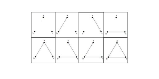
The degree (or order) of a vertex in a graph is the number of edges with that vertex as an end point. A vertex whose degree is an even number is said to have an even degree or even vertex .

The in-degree of a vertex in a directed graph is the number of edges with that vertex as an end point. The out-degree of a vertex in a directed graph is the number of edges with that vertex as a starting point.

A  graph having no edges  is called a Null Graph.

A simple graph with ‘n’ mutual vertices is called a complete graph and it is  denoted by ‘K n ’ . In the graph,  a vertex should have edges with all other vertices,  then it called a complete graph.

In other words, if a vertex is connected to all other vertices in a graph, then it is called a complete graph.

A simple graph G = (V, E) with vertex partition V = {V 1 , V 2 } is called a bipartite graph  if every edge of E joins a vertex in V 1  to a vertex in V 2 .

In general, a Bipartite graph has two sets of vertices, let us say, V 1  and V 2 , and if an edge is drawn, it should connect any vertex in set V 1  to any vertex in set V 2 .

A bipartite graph ‘G’, G = (V, E) with partition V = {V 1 , V 2 } is said to be a complete bipartite graph if every vertex in V 1  is connected to every vertex of V 2 .

In general, a complete bipartite graph connects each vertex from set V 1  to each vertex from set V 2 .

Example: The following graph is a complete bipartite graph because it has edges connecting each vertex from set V 1  to each vertex from set V 2 .

If |V 1 | = m and |V 2 | = n, then the complete bipartite graph is denoted by K m, n .

• K m,n has (m+n) vertices and (mn) edges.
• K m,n is a regular graph if m=n.

In general,  a complete bipartite graph is not a complete graph . K m,n  is a complete graph if m=n=1. The maximum number of edges in a bipartite graph with  n  vertices is n 2 /4 If n = 10, k5, 5 = n 2 /4 = 100/4 = 25 Similarly, K6, 4 = 24 K7, 3 = 21 K8, 2 = 16 K9, 1 = 9

If n = 9, k5, 4 = n 2 /4 = 81/4 = 20 Similarly, K6, 3 = 18 K7, 2 = 14 K8, 1 = 8

‘G’ is a bipartite graph if ‘G’ has no cycles of odd length. A special case of bipartite graph is a  star graph .

GRAPH REPRESENTATION

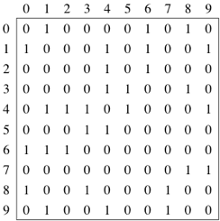
Adjacency matrices.

For a graph with |V| vertices, an  adjacency matrix  is a ∣V∣×∣V∣ matrix of 0s and 1s, where the entry in row i and column j is 1 if and only if the edge (i, j) is in the graph. If you want to indicate an edge weight, put it in the row i, column j entry, and reserve a special value (perhaps null) to indicate an absent edge. Here’s the adjacency matrix for the social network graph:

INCIDENCE MATRICES

Let G be a graph with n vertices, m edges and without self-loops. The incidence matrix A of G is an n × m matrix A = [a ij ] whose n rows correspond to the n vertices and the m columns correspond to m edges such that: a i,j = 1 if jth edge m j is incident on the i th vertex else it’s 0.

TRANSITION MATRICES

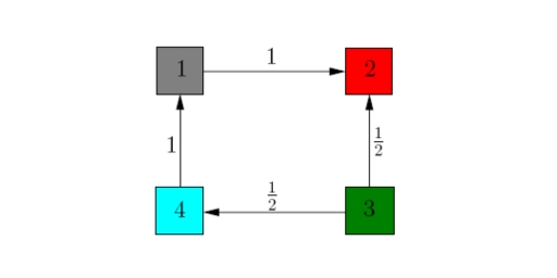
Example: Then the transition matrix associated to it is:

In general, a matrix is called  primitive  if there is a positive integer k such that A k  is a positive matrix. A graph is called  connected  if for any two different nodes i and j there is a directed path either from i to j or from j to i. On the other hand, a graph is called  strongly connected  if starting at any node i we can reach any other different node j by walking on its edges.

The direction of movement in a transition matrix is opposite to that of an adjacency matrix.

THE MINIMUM SPANING TREE

Given an undirected and connected graph G = (V, E), a spanning tree of the graph G is a tree that spans G (that is, it includes every vertex of G) and is a subgraph of G (every edge in the tree belongs to G)

The cost of the spanning tree is the sum of the weights of all the edges in the tree. There can be many spanning trees. Minimum spanning tree is the spanning tree where the cost is minimum among all the spanning trees. There also can be many minimum spanning trees.

Minimum spanning tree has direct application in the design of networks. It is used in algorithms approximating the travelling salesman problem , multi-terminal minimum cut problem and minimum-cost weighted perfect matching.

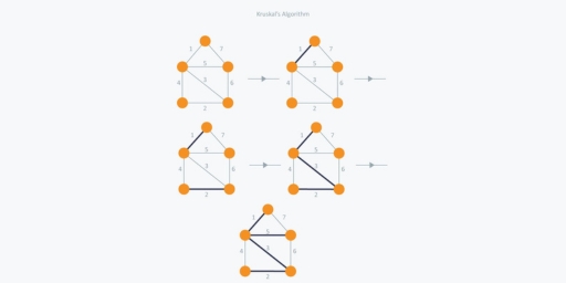
KRUSHKAL’S ALGORITHM

Kruskal’s Algorithm builds the spanning tree by adding edges one by one into a growing spanning tree. Kruskal’s algorithm follows greedy approach as in each iteration it finds an edge which has least weight and add it to the growing spanning tree.

Algorithm Steps:

• Sort the graph edges with respect to their weights.
• Start adding edges to the MST from the edge with the smallest weight until the edge of the largest weight.
• Only add edges which doesn’t form a cycle, edges which connect only disconnected components.

PRIM’S ALGORITHM

Prim’s Algorithm also use Greedy approach to find the minimum spanning tree. In Prim’s Algorithm we grow the spanning tree from a starting position. Unlike an  edge  in Kruskal’s, we add  vertex  to the growing spanning tree in Prim’s.

• Maintain two disjoint sets of vertices. One containing vertices that are in the growing spanning tree and other that are not in the growing spanning tree.
• Select the cheapest vertex that is connected to the growing spanning tree and is not in the growing spanning tree and add it into the growing spanning tree. This can be done using Priority Queues. Insert the vertices, that are connected to growing spanning tree, into the Priority Queue.
• Check for cycles. To do that, mark the nodes which have been already selected and insert only those nodes in the Priority Queue that are not marked.

THE CHINESE POSTMAN PROBLEM

A connected graph G is Eulerian if there exists a closed trail containing every edge of G. Such a trail is an Eulerian trail . Note that this definition requires each edge to be traversed once and once only, A non-Eulerian graph G is semi-Eulerian if there exists a trail containing every edge of G.

A trail is walk that repeats no edges. A circuit is a trail that starts and finishes at the same vertex.

The problem is how to find a shortest closed walk of the graph in which each edge is traversed at least once, rather than exactly once. In graph theory, an Euler cycle in a connected, weighted graph is called the Chinese Postman problem .

To find a minimum Chinese postman route we must walk along each edge at least once and in addition we must also walk along the least pairings of odd vertices on one extra occasion. An algorithm for finding an optimal Chinese postman route is:

• List all odd vertices.
• List all possible pairings of odd vertices.
• For each pairing find the edges that connect the vertices with the minimum weight.
• Find the pairings such that the sum of the weights is minimised.
• On the original graph add the edges that have been found in Step 4.
• The length of an optimal Chinese postman route is the sum of all the edges added to the total found in Step 4.
• A route corresponding to this minimum weight can then be easily found.

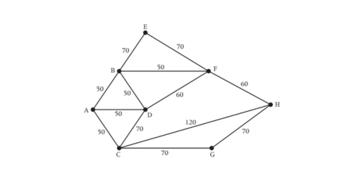
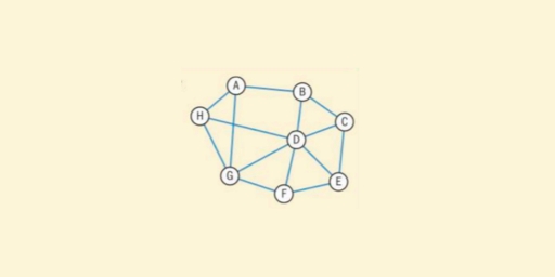
• The odd vertices are A and H.
• There is only one way of pairing these odd vertices, namely AH.
• The shortest way of joining A to H is using the path AB, BF, FH, a total length of 160.

• The length of the optimal Chinese postman route is the sum of all the edges in the original network, which is 840 m, plus the answer found in Step 4, which is 160 m. Hence the length of the optimal Chinese postman route is 1000 m.
• One possible route corresponding to this length is ADCGHCABDFBEFHFBA, but many other possible routes of the same minimum length can be found.

TRAVELLING SALESMAN PROBLEM

A path is a walk which does not pass through any vertex more than once. A cycle is a walk that begins and ends at the same vertex, but otherwise does not pass through any vertex more than once.

A Hamiltonian path or cycle is a path or cycle which passes through all the vertices in a graph.

The classical travelling salesman problem (TSP) is to find the Hamiltonian cycle of least weight in a complete weighted graph.

The practical TSP is to find the walk of least weight that passes through each vertex of a graph. In this case the graph need not be complete.

Suppose a salesman wants to visit a certain number of cities allotted to him. He knows the distance of the journey between every pair of cities. His problem is to select a route the starts from his home city, passes through each city exactly once and return to his home city the shortest possible distance. This problem is closely related to finding a Hamiltonian circuit of minimum length. If we represent the cities by vertices and road connecting two cities edges we get a weighted graph where, with every edge e i  a number w i (weight) is associated.

A physical interpretation of the above abstract is: consider a graph G as a map of n cities where w (i, j) is the distance between cities i and j. A salesman wants to have the tour of the cities which starts and ends at the same city includes visiting each of the remaining a cities once and only once.

In the graph, if we have n vertices (cities), then there is (n-1)! Edges (routes) and the total number of Hamiltonian circuits in a complete graph of n vertices will be (n – 1)!/2

FINDING AN UPPER BOUND

An upper bound can be found using the nearest neighbour algorithm :

Step1:  Select an arbitrary vertex and find the vertex that is nearest to this starting vertex to form an initial path of one edge.

Step2:  Let v denote the latest vertex that was added to the path. Now, among the result of the vertices that are not in the path, select the closest one to v and add the path, the edge-connecting v and this vertex. Repeat this step until all the vertices of graph G are included in the path.

Step3:  Join starting vertex and the last vertex added by an edge and form the circuit.

This will always produce a valid Hamiltonian cycle , and therefore must be at least as long as the minimum cycle . Hence, it is an upper bound. By choosing different starting vertices, a number of different upper bounds can be found.

The best upper bound is the upper bound with the smallest value.

FINDING A LOWER BOUND

Lower bounds can be found by using spanning trees . Since removal of one edge from any Hamilton cycle yields a spanning tree, we see that solution to TSP > minimum length of a spanning tree (MST) .

Consider any vertex v in the graph G. Any Hamilton cycle in G has to consist of two edges from v, say vu and vw, and a path from u to w in the graph G \ {v} obtained from G by removing v and its incident edges. Since this path is a spanning tree of G \ {v}, we have Solution to TSP ≥ (sum of lengths of two shortest edges from v) + (MST of G \ {v}).

An alternative is to use the deleted vertex algorithm .

The method for finding a lower bound:

• Delete a vertex and find the minimum spanning tree for what remains.
• Reconnect the vertex you deleted using the two smallest arcs.
• Repeat this process for all vertices and select the highest as the best lower bound.

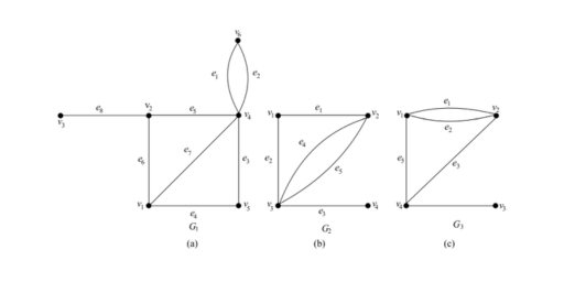
Example 1: Use the nearest-neighbour method to solve the following travelling salesman problem, for the graph shown in fig starting at vertex v 1 .

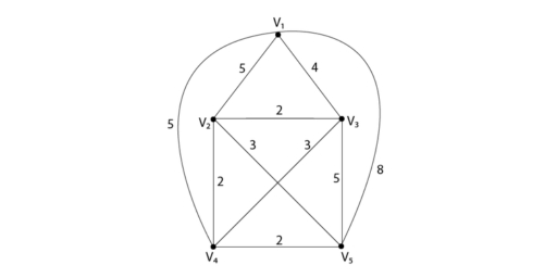
The total distance of this route is 18.

This has weight = 25.

Lower bound = 25 + 5 + 4 = 34

We Are Here To Help You To Excel in Your Exams!

Book your free demo session now, head office.

• HD-213, WeWork DLF Forum, Cyber City, DLF Phase 3, DLF, Gurugram, Haryana-122002
• +919540653900
• [email protected]

Tychr Online Tutors

IB Online Tutor

Cambridge Online Tutor

Edexcel Online Tutors

AQA Online Tutors

OCR Online Tutors

AP Online Tutors

SAT Online Tuition Classes

ACT Online Tuition Classes

IB Tutor in Bangalore

IB Tutors In Mumbai

IB Tutors In Pune

IB Tutors In Delhi

IB Tutors In Gurgaon

IB Tutors In Noida

IB Tutors In Chennai

Quick Links

Who We Are?

Meet Our Team

Our Results

Our Testimonials

Let’s Connect!

Terms & Conditions

Privacy Policy

Refund Policy

Recent Articles

Inside gwu: george washington university admissions, inside brown university: demystifying admission requirements, emerson college admission requirements: a closer look, bowdoin admission requirements: your path to excellence, international ib tutors.

IB Tutor in Singapore

IB Tutor in Toronto

IB Tutor in Seattle

IB Tutor in San Diego

IB Tutor in Vancouver

IB Tutor in London

IB Tutor in Zurich

IB Tutor in Basel

IB Tutor in Lausanne

IB Tutor in Geneva

IB Tutor in Ontario

IB Tutor in Boston

IB Tutor in Kowloon

IB Tutor in Hong Kong

IB Tutor in San Francisco

IB Tutor in Dallas

IB Tutor in Houston

IB Tutor in Chicago

IB Tutor in New York City

IB Tutor in Brooklyn

IB Tutor in Washington

IB Tutor in Berkshire

IB Tutor in Sussex

IB Tutor in Melbourne

IB Tutor in Western Australia

Ⓒ 2023 TYCHR ACADEMY | All Rights Reserved

Download Our selected list of 30+ IB IA Ideas for FREE!

ANNOUNCEMENT

Download our Successful College Application Guide developed by counselors from the University of Cambridge for institutions like Oxbridge  alongside other Ivy Leagues . To join our college counseling program, call at +918825012255

We are hiring a Business Development Associate and Content Writer and Social Media Strategist at our organisation TYCHR to take over the responsibility of conducting workshops and excelling in new sales territory. View More

We will keep fighting for all libraries - stand with us!

Internet Archive Audio

• This Just In
• Grateful Dead
• Old Time Radio
• 78 RPMs and Cylinder Recordings
• Audio Books & Poetry
• Computers, Technology and Science
• Music, Arts & Culture
• News & Public Affairs
• Spirituality & Religion
• Radio News Archive

• Flickr Commons
• Occupy Wall Street Flickr
• NASA Images
• Solar System Collection
• Ames Research Center

• All Software
• Old School Emulation
• MS-DOS Games
• Historical Software
• Classic PC Games
• Software Library
• Kodi Archive and Support File
• Vintage Software
• CD-ROM Software
• CD-ROM Software Library
• Software Sites
• Tucows Software Library
• Shareware CD-ROMs
• Software Capsules Compilation
• CD-ROM Images
• ZX Spectrum
• DOOM Level CD

• Smithsonian Libraries
• FEDLINK (US)
• Lincoln Collection
• American Libraries
• Canadian Libraries
• Universal Library
• Project Gutenberg
• Children's Library
• Biodiversity Heritage Library
• Books by Language
• Additional Collections

• Prelinger Archives
• Democracy Now!
• Occupy Wall Street
• TV NSA Clip Library
• Animation & Cartoons
• Arts & Music
• Computers & Technology
• Cultural & Academic Films
• Ephemeral Films
• Sports Videos
• Videogame Videos
• Youth Media

Search the history of over 866 billion web pages on the Internet.

Mobile Apps

• Wayback Machine (iOS)
• Wayback Machine (Android)

Browser Extensions

Archive-it subscription.

• Explore the Collections
• Build Collections

Save Page Now

Capture a web page as it appears now for use as a trusted citation in the future.

Please enter a valid web address

• Donate Donate icon An illustration of a heart shape

In pursuit of the traveling salesman : mathematics at the limits of computation

Bookreader item preview, share or embed this item, flag this item for.

• Graphic Violence
• Explicit Sexual Content
• Hate Speech
• Misinformation/Disinformation
• Marketing/Phishing/Advertising
• Misleading/Inaccurate/Missing Metadata

plus-circle Add Review comment Reviews

8 Favorites

Better World Books

DOWNLOAD OPTIONS

No suitable files to display here.

IN COLLECTIONS

Uploaded by station09.cebu on March 27, 2023

SIMILAR ITEMS (based on metadata)