travelling salesman application

Travelling Salesman Problem: Python, C++ Algorithm

What is the Travelling Salesman Problem (TSP)?

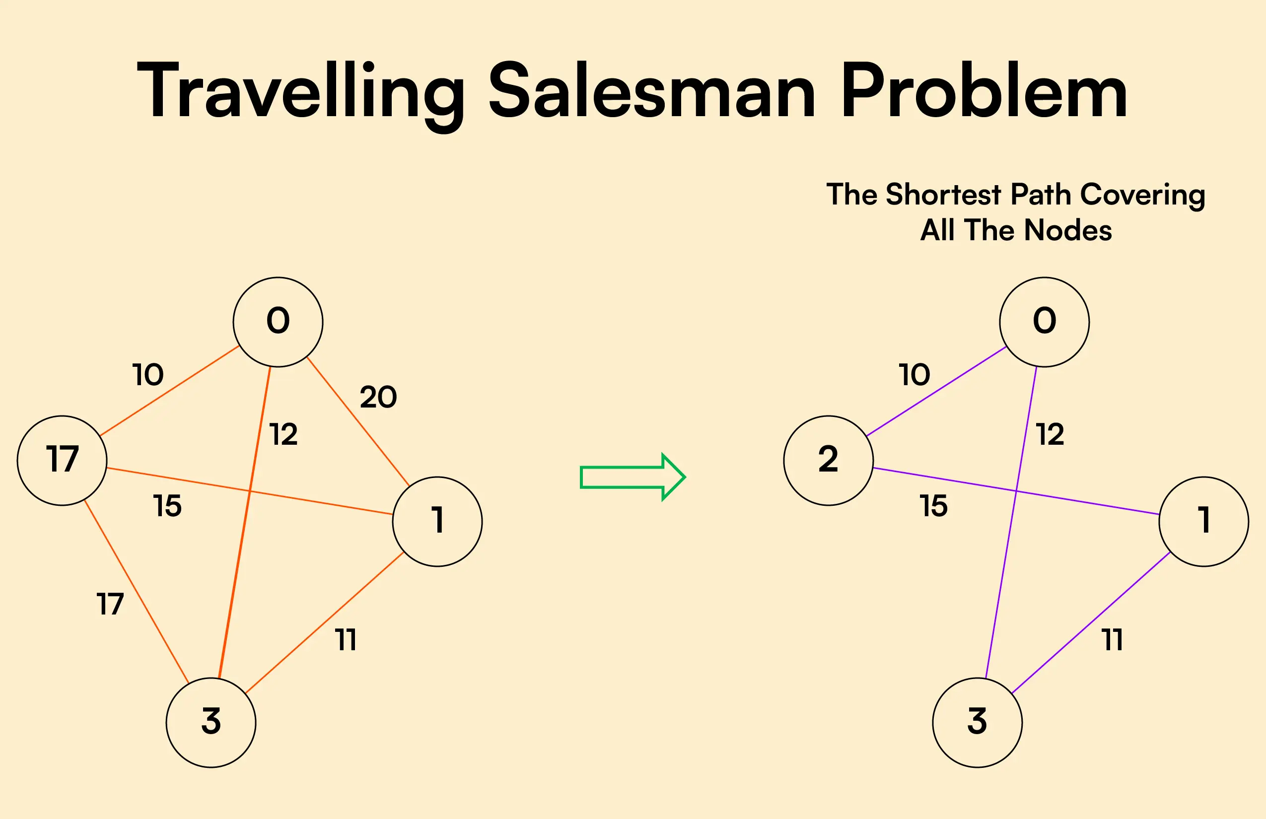
Travelling Salesman Problem (TSP) is a classic combinatorics problem of theoretical computer science. The problem asks to find the shortest path in a graph with the condition of visiting all the nodes only one time and returning to the origin city.

The problem statement gives a list of cities along with the distances between each city.

Objective: To start from the origin city, visit other cities only once, and return to the original city again. Our target is to find the shortest possible path to complete the round-trip route.

Example of TSP

Here a graph is given where 1, 2, 3, and 4 represent the cities, and the weight associated with every edge represents the distance between those cities.

The goal is to find the shortest possible path for the tour that starts from the origin city, traverses the graph while only visiting the other cities or nodes once, and returns to the origin city.

For the above graph, the optimal route is to follow the minimum cost path: 1-2-4-3-1. And this shortest route would cost 10+25+30+15 =80

Different Solutions to Travelling Salesman Problem

Travelling Salesman Problem (TSP) is classified as a NP-hard problem due to having no polynomial time algorithm. The complexity increases exponentially by increasing the number of cities.

There are multiple ways to solve the traveling salesman problem (tsp). Some popular solutions are:

The brute force approach is the naive method for solving traveling salesman problems. In this approach, we first calculate all possible paths and then compare them. The number of paths in a graph consisting of n cities is n! It is computationally very expensive to solve the traveling salesman problem in this brute force approach.

The branch-and-bound method: The problem is broken down into sub-problems in this approach. The solution of those individual sub-problems would provide an optimal solution.

This tutorial will demonstrate a dynamic programming approach, the recursive version of this branch-and-bound method, to solve the traveling salesman problem.

Dynamic programming is such a method for seeking optimal solutions by analyzing all possible routes. It is one of the exact solution methods that solve traveling salesman problems through relatively higher cost than the greedy methods that provide a near-optimal solution.

The computational complexity of this approach is O(N^2 * 2^N) which is discussed later in this article.

The nearest neighbor method is a heuristic-based greedy approach where we choose the nearest neighbor node. This approach is computationally less expensive than the dynamic approach. But it does not provide the guarantee of an optimal solution. This method is used for near-optimal solutions.

Algorithm for Traveling Salesman Problem

We will use the dynamic programming approach to solve the Travelling Salesman Problem (TSP).

Before starting the algorithm, let’s get acquainted with some terminologies:

A graph G=(V, E), which is a set of vertices and edges.
V is the set of vertices.
E is the set of edges.
Vertices are connected through edges.
Dist(i,j) denotes the non-negative distance between two vertices, i and j.

Let’s assume S is the subset of cities and belongs to {1, 2, 3, …, n} where 1, 2, 3…n are the cities and i, j are two cities in that subset. Now cost(i, S, j) is defined in such a way as the length of the shortest path visiting node in S, which is exactly once having the starting and ending point as i and j respectively.

For example, cost (1, {2, 3, 4}, 1) denotes the length of the shortest path where:

Starting city is 1
Cities 2, 3, and 4 are visited only once
The ending point is 1

The dynamic programming algorithm would be:

Set cost(i, , i) = 0, which means we start and end at i, and the cost is 0.
When |S| > 1, we define cost(i, S, 1) = ∝ where i !=1 . Because initially, we do not know the exact cost to reach city i to city 1 through other cities.
Now, we need to start at 1 and complete the tour. We need to select the next city in such a way-

cost(i, S, j)=min cost (i, S−{i}, j)+dist(i,j) where i∈S and i≠j

For the given figure, the adjacency matrix would be the following:

Algorithm for Traveling Salesman Problem

Let’s see how our algorithm works:

Step 1) We are considering our journey starting at city 1, visit other cities once and return to city 1.

Step 2) S is the subset of cities. According to our algorithm, for all |S| > 1, we will set the distance cost(i, S, 1) = ∝. Here cost(i, S, j) means we are starting at city i, visiting the cities of S once, and now we are at city j. We set this path cost as infinity because we do not know the distance yet. So the values will be the following:

Cost (2, {3, 4}, 1) = ∝ ; the notation denotes we are starting at city 2, going through cities 3, 4, and reaching 1. And the path cost is infinity. Similarly-

cost(3, {2, 4}, 1) = ∝

cost(4, {2, 3}, 1) = ∝

Step 3) Now, for all subsets of S, we need to find the following:

cost(i, S, j)=min cost (i, S−{i}, j)+dist(i,j), where j∈S and i≠j

That means the minimum cost path for starting at i, going through the subset of cities once, and returning to city j. Considering that the journey starts at city 1, the optimal path cost would be= cost(1, {other cities}, 1).

Let’s find out how we could achieve that:

Now S = {1, 2, 3, 4}. There are four elements. Hence the number of subsets will be 2^4 or 16. Those subsets are-

1) |S| = Null:

2) |S| = 1:

{{1}, {2}, {3}, {4}}

3) |S| = 2:

{{1, 2}, {1, 3}, {1, 4}, {2, 3}, {2, 4}, {3, 4}}

4) |S| = 3:

{{1, 2, 3}, {1, 2, 4}, {2, 3, 4}, {1, 3, 4}}

5) |S| = 4:

As we are starting at 1, we could discard the subsets containing city 1.

The algorithm calculation:

1) |S| = Φ:

cost (2, Φ, 1) = dist(2, 1) = 10

cost (3, Φ, 1) = dist(3, 1) = 15

cost (4, Φ, 1) = dist(4, 1) = 20

cost (2, {3}, 1) = dist(2, 3) + cost (3, Φ, 1) = 35+15 = 50

cost (2, {4}, 1) = dist(2, 4) + cost (4, Φ, 1) = 25+20 = 45

cost (3, {2}, 1) = dist(3, 2) + cost (2, Φ, 1) = 35+10 = 45

cost (3, {4}, 1) = dist(3, 4) + cost (4, Φ, 1) = 30+20 = 50

cost (4, {2}, 1) = dist(4, 2) + cost (2, Φ, 1) = 25+10 = 35

cost (4, {3}, 1) = dist(4, 3) + cost (3, Φ, 1) = 30+15 = 45

cost (2, {3, 4}, 1) = min [ dist[2,3]+Cost(3,{4},1) = 35+50 = 85,

dist[2,4]+Cost(4,{3},1) = 25+45 = 70 ] = 70

cost (3, {2, 4}, 1) = min [ dist[3,2]+Cost(2,{4},1) = 35+45 = 80,

dist[3,4]+Cost(4,{2},1) = 30+35 = 65 ] = 65

cost (4, {2, 3}, 1) = min [ dist[4,2]+Cost(2,{3},1) = 25+50 = 75

dist[4,3]+Cost(3,{2},1) = 30+45 = 75 ] = 75

cost (1, {2, 3, 4}, 1) = min [ dist[1,2]+Cost(2,{3,4},1) = 10+70 = 80

dist[1,3]+Cost(3,{2,4},1) = 15+65 = 80

dist[1,4]+Cost(4,{2,3},1) = 20+75 = 95 ] = 80

So the optimal solution would be 1-2-4-3-1

Pseudo-code

Implementation in c/c++.

Here’s the implementation in C++ :

Implementation in Python

Academic solutions to tsp.

Computer scientists have spent years searching for an improved polynomial time algorithm for the Travelling Salesman Problem. Until now, the problem is still NP-hard.

Though some of the following solutions were published in recent years that have reduced the complexity to a certain degree:

The classical symmetric TSP is solved by the Zero Suffix Method.
The Biogeography‐based Optimization Algorithm is based on the migration strategy to solve the optimization problems that can be planned as TSP.
Multi-Objective Evolutionary Algorithm is designed for solving multiple TSP based on NSGA-II.
The Multi-Agent System solves the TSP of N cities with fixed resources.

Application of Traveling Salesman Problem

Travelling Salesman Problem (TSP) is applied in the real world in both its purest and modified forms. Some of those are:

Planning, logistics, and manufacturing microchips : Chip insertion problems naturally arise in the microchip industry. Those problems can be planned as traveling salesman problems.
DNA sequencing : Slight modification of the traveling salesman problem can be used in DNA sequencing. Here, the cities represent the DNA fragments, and the distance represents the similarity measure between two DNA fragments.
Astronomy : The Travelling Salesman Problem is applied by astronomers to minimize the time spent observing various sources.
Optimal control problem : Travelling Salesman Problem formulation can be applied in optimal control problems. There might be several other constraints added.

Complexity Analysis of TSP

So the total time complexity for an optimal solution would be the Number of nodes * Number of subproblems * time to solve each sub-problem. The time complexity can be defined as O(N 2 * 2^N).

Space Complexity: The dynamic programming approach uses memory to store C(S, i), where S is a subset of the vertices set. There is a total of 2 N subsets for each node. So, the space complexity is O(2^N).

Next, you’ll learn about Sieve of Eratosthenes Algorithm

Linear Search: Python, C++ Example
DAA Tutorial PDF: Design and Analysis of Algorithms
Heap Sort Algorithm (With Code in Python and C++)
Kadence’s Algorithm: Largest Sum Contiguous Subarray
Radix Sort Algorithm in Data Structure
Doubly Linked List: C++, Python (Code Example)
Singly Linked List in Data Structures
Adjacency List and Matrix Representation of Graph

What Is A Travelling Salesman Problem (TSP)?

Published Date: March 2, 2024

Table of Contents

The majority of field salespeople get up in the morning only having a general notion of what to do to make the best possible use of their workday. They want to reach multiple customers, as well as others along their journey that they are unaware of, however they might not follow a well-planned timetable. This weakness results in either retracing or getting out of time. The lack of sales route planning delays client meetings and missed opportunities.

Consider a salesperson who wants to go to several cities, but desires to cover as few miles as possible and come back to where they started. The Travelling Salesman Problem (TSP), a widely recognized problem, has remained the subject of research for more than a century. Finding the lowest possible weight Hamiltonian cycle that keeps both the travel expenses and the amount of distance travelled to a minimum is the salesman’s goal in the TSP.

The task of determining the shortest possible path or route for the salesman to travel provided a starting point, several cities (nodes), as well as a finishing point, is known as the “Travelling Salesman Problem” (TSP). This is a typical computational problem in fieldwork that could cause monetary damage and disrupt several field processes.

TSP occurs when there are several routes accessible but it is very difficult for you or the traveller to select the one with the lowest cost. By utilizing route optimization techniques to identify more profitable routes, field businesses can lower the release of greenhouse gases by travelling shorter distances.

What Is The History Of Travelling Salesman Problem?

The Travelling Salesman Problem, or TSP, has its roots at the beginning of the nineteenth century, but Merrill M. Flood was the first person to formalize it mathematically in 1930 while trying to figure out a school bus routing problem. The term “TSP” was first used in a 1949 RAND Corporation paper. It was then used by Hassler Whitney at Princeton under the title of the “48 states problem,” which meant the shortest path was examined for travelling all of the surrounding 48 United States.

The challenge of a salesperson travelling to several locations in the shortest amount of time, spending the smallest sum of money, and covering the shortest distance is only one aspect of TSP. The world is currently preparing for the fourth industrial revolution that will result in it. As advanced technology is included in the manufacturing process, TSP offers access to a broad range of functions. For example, a form of TSP could aid in the construction of an effective microprocessor. Analogously, by changing the location of colors, an asymmetric form of TSP can optimize the cost of setting up of a paint production unit.

Major Challenges Of Travelling Salesman Problem

When salespeople wake up, nearly every one of them considers how to best utilize their workday. They have a great deal of planned appointments as well as many impromptu ones with their clients. Being a salesperson is challenging since your daily routine will inevitably provide you with a number of obstacles. Some of the travelling salesmen challenges are:

First of all, salesmen are under constant time limitations as they complete numerous deliveries in a condensed amount of time each day. They must arrange their routes to maximize their potential in order to get around this.
The work schedules of salesmen are typically flexible. This defect commonly forces salespeople to go back and forth between their steps and take longer routes in order to get to client locations. This absence of planning for the journey leads to lost meetings and chances.
The salesperson nowadays faces road congestion, last-minute client demands, and tight delivery window timings along with the travel challenges that beset those before them.
Parallel to how salespeople modify their routes on the spot, the route algorithm needs to be adaptable and quick to sudden occurrences like traffic jams, automobile failures, and volume spikes. A TSP solution needs to be able to deal with complicated networks and huge databases with ease.
The number of routes grows dramatically in tandem with the number of destinations. The computing power of even the most advanced systems is surpassed by this hyperbolic development.

5 Most Reliable And Successful Solutions For The Travelling Salesman Problem

Since the first brute force technique was developed in the 1950s, TSP techniques have remained in use. Further refined methods like nearest neighbor algorithms and dynamic programming have been created since then. With the aid of all of these sophisticated algorithms, researchers and developers can now solve the TSP almost with the same speed and efficiency as they did before. One can solve the TSP in a much less amount of time by utilizing these algorithms.

The Brute Force Approach

In order to find the shortest distinct solution, the Brute Force method, sometimes referred to as the Naive Method, computes and contrasts each potential set of paths or routes. One has to first figure out the overall amount of routes, then sketch and list every feasible route in order to resolve the TSP employing the Brute-Force method. The best course of action is to determine each route’s distance and then select the one that is the shortest. This is rarely helpful outside of conceptual computing seminars and is only practical for small issues.

The Nearest Neighbour Approach

The most basic way to resolve the TSP is with this approach. This approach usually starts from the closest location, visiting all other locations, and then returning to the initial location. The following are the steps needed to solve the TSP employing the Nearest Neighbour approach:

Select an arbitrary location.
Find the closest unexplored location and get there.
The salesperson needs to go back to the starting point after visiting each location.

The Branch And Bound Approach

Determining the least cost for the rest of the routes that the beginning stages of methods such as the brute-force approach give is the focus of the branch and bound approach. Also known as Parallel TSP, this approach makes the assumption that we don’t wish to attempt every “possible” path. Even applying logic would likely help to simplify it.

We won’t, for instance, travel to the drop-off location that is the longest distance before we head back to the location that is closest to the warehouse. With the use of nodes and “costs” associated with each node, the approach calculates the likelihood that a particular option will result in a problem-solving solution.

Dynamic Programming

Dynamic programming is a method for handling intricate issues by breaking them down into smaller, easier-to-handle subproblems and addressing each one separately. It can find the shortest path that covers each city precisely once and avoids doing duplicate computations, which is why it is frequently used to solve the Travelling Salesman Problem. Because the method of dynamic programming can be utilized for solving issues of any size, it is more versatile than the brute force approach. Dynamic programming does have certain restrictions, though. It can be time-consuming and operationally costly because it requires the solution of a large number of smaller issues.

What Are Real-Time Travelling Salesman Problem Applications?

A widely recognized optimization problem with many practical applications across many industries is the travelling salesman problem (TSP). Every one of these practical uses exemplifies the TSP’s adaptability and the various challenges it has been used to tackle. Following are some of the TSP’s more noteworthy uses:

Vehicle Routing: Delivery and distribution route optimization is a common application of the TSP. Locations in this application correlate to delivery sites, and the salesperson is symbolized by a delivery vehicle. The idea is to determine the shortest path that makes precisely one stop at each destination before returning to the initial location. This issue is crucial in the world of delivery firms because it allows them to minimize fuel use, lower the number of vehicles needed, and guarantee the on-time distribution of products.

Logistics And Manufacturing: In the transportation and logistics sector, where businesses must optimize their supply routes to lower expenses and boost efficacy, the TSP is a prevalent issue. For instance, in order to save petrol and delivery time, a delivery service could have to determine the shortest path that stops at every one of its clients in a certain location.

The TSP is also applicable to production and manufacturing scheduling, as these fields require businesses to optimize their manufacturing processes to save expenses and boost productivity. For instance, in order to reduce downtime and increase production, a manufacturing facility may need to determine the quickest path to all of the machinery that requires maintenance.

Network Design And Optimization : In network architecture and optimization, the TSP is employed by businesses to optimize the flow of data, products, or services among a network of nodes. For instance, in order to reduce the loss of signal and enhance network efficiency, a telecommunications provider might need to determine the shortest path between its network nodes.

Circuit Design: The TSP is utilized in the area of electronics to create effective circuit schematics. In this case, the salesperson is the electrical signal that must pass via each city precisely once, and the cities are the circuit’s constituent parts. The objective is to determine the shortest path that minimizes the entire circuit’s resistance and impedance.

Robotics And Automation: The TSP also has applications in the fields of automation and robotics, where businesses must maximize machine or robot motion in order to cut expenses and boost productivity. For instance, in order to do different duties like choosing and arranging products or examining machinery, a robot might be required to determine the shortest route to take to every site in a plant.

How TSP Solves Last-Mile Delivery Problems?

The last step in a supply chain is the focus of the last-mile delivery issue. It entails moving cargo from a central point of transportation, like a terminal or warehouse, to the final destination.

Inadequate Route Planning
Delivery Windows
Traffic Congestions
High Travel/Fuel Costs
Late/Untimely Deliveries

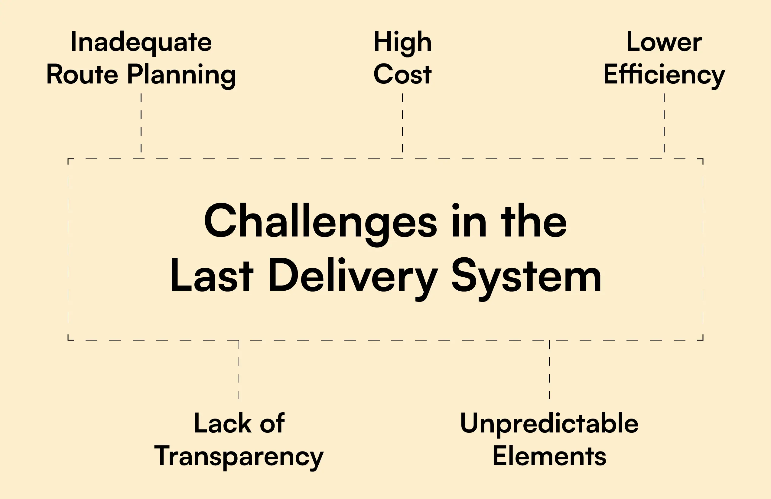
By streamlining routes for delivery, cutting down on stops, and minimizing the total kilometers travelled, TSP solutions are essential in tackling this problem. The Travelling Salesman Problem yields effective solutions that optimize and reduce last-mile delivery costs. These technologies assist delivery companies in identifying a series of courses or routes that minimize delivery expenses. A number of delivery destinations, warehouse locations, and delivery automobiles are all part of the delivery issue arena.

How AI Helps In Solving Travelling Salesman Problem (TSP)?

Artificial intelligence (AI) methods including neural networks, genetic algorithms, and ant colony optimization were all used to solve the TSP effectively. Supply chain management and logistics have benefited greatly from AI. This involves enhancing transportation routes or reducing the amount of miles driven when delivering products. The use of artificial intelligence assists business operational leaders in creating and allocating the best possible sales plans for their employees. It provides the best possible meeting plans by accounting for factors such as proximity, automobile capacity, client time window, salespeople’s abilities, driver skills, and many more.

We can anticipate significantly more advanced applications in TSP solutions given the swift development in AI. This might entail the creation of novel artificial intelligence methods that can deal with bigger and more complicated problems or the application of quantum algorithms for faster resolution. The development of AI has revolutionized the way we approach and deal with these issues, increasing productivity and effectiveness across a range of businesses. We do not doubt that AI will play a substantially greater role in resolving TSP and related issues as the technology develops.

The Travelling Salesman Problem is a complex statistical puzzle that simulates the daily activities of a salesperson. It describes the endeavors of a door-to-door salesperson who is attempting to determine the most efficient and/or fastest manner to complete all of the locations on their list of visits in a specific amount of time (often a workday). Initially, it used to be a salesperson’s issue, but far more people deal with it nowadays.

Field workers can learn about optimization concepts and use them when dealing with a range of real-world issues through exploring the TSP. Even though the TSP is still a difficult issue, advances in computer technology and algorithms have made it easier to get to and solve. In the end, solving the TSP along with other challenging optimization issues can enhance both our personal life and the world that we dwell in.

Related Blogs

Explaining Sales Competency Framework And Its Essential Skills In Sales

Top 20 Sales Blogs To Follow In 2024

Top 10 Sales Conferences For Salespersons To Attend In 2024

A Detailed Brief On Daily Sales Reports

10 Typical Sales Commission Structures with Formulas and Examples

Inside Sales Vs Outside Sales

A Definitive Guide To SaaS Sales In 2023

A Detailed Brief About Sales Performance Management

10 Best Sales Podcasts For Inside And Outside Reps

12 Effective Sales Appointment Setting Tips

How to increase sales of a new product in field sales?

How to Create Steps for an Automated Field Sales Funnel

How to classify and identify potential leads

7 Best Sales Mapping Software For Your Business

How To Prepare Effectively For A Client Sales Meetings?

A complete guide on how AI helps your Sales Business to grow?

A Brief Guide On Soft Selling And Its Techniques

A Detailed Brief On The Buyer’s Journey In Sales

How to setup B2B Sales funnels And Strategies

10 Sales Conferences Every Salesperson Should Attend In 2023

How To Write Sales Follow-Up Emails After No Response With Sample Email Templates

Important Field Sales KPIs Every Sales Manager Should Know

What Is Sales Data: Importance And Types Of Sales Data Reports

A Brief Knowledge On Sales Analysis: How To Perform An Effective Sales Analysis?

7 Constructive Field Sales Canvassing Tips For 2024

How to set up a successful sales management process?

8 Productive Tips For Field Sales Reps To Generate More Leads

10 Best Ways To Boost Employee Engagement And Motivation

7 Best Advanced Sales Training Program To Upgrade Your Sales Career

How To Prepare Yourself For A Sales Supervisor Job Interview

12 Best AI Tools to Increase the Sales of Your Business

8 Best Practices For Keeping An Organized Sales Pipeline

10 Books That Well Help You To Become A Better Salesperson

Top 20 sales blogs to follow in 2023

How Can Salespeople Improve Their Chances Of Getting An Appointment?

A complete guide on solar sales- Tips to improve solar sales

How Does A Blog Directly Impact The Business Of A Company

How to resolve the conflict between your Sales and Marketing Teams

A Brief Guide To Sales Methodology: Best Sales Methodologies For Your Team

How to handle objections in sales

10 Best Sales Enablement Tools In 2023

How to use the right tone and tonality in sales.

10 best sales closing techniques for salespeople

How to plan a commission structure for your salespeople

How to plan a 30 60 90 sales plan with an example

Importance of Regression Analysis in sales forecasting

Importance of Open-Ended Questions in sales

How to Plan for a New Sales Territory

A Complete Guide On Door-To-Door Sales: Tips For Effective Door-To-Door Selling

How to Improve customer service mindset for your Staff

What Is Sales Volume And How To Use Sales Volume Effectively To Get Revenue

5 Best Task Management Software For Field Employees

How To Set Sales Targets For Your Team: 6 Sales Target Tips To Follow

How To Make A Sales Team More Productive: 8 Tips To Follow

How To Boost Sales For A Small Business In 2022

10 Tips to Increase Your Collection Agent Performance

Top 25 Team Motivational Quotes For Better Productivity

8 Essential Team Management Skills Every Manager Must Know

How To Track Sales Person Of Your Organization

How To Prioritize Your Leads Or Prospects In Sales

5 Most Common Myths Related To Employee Management

How To Stay Focused At Work: 6 Ways That Can Increase Field Employee Productivity

5 Best Ways To Start A Good Sales Conversation With Any Prospect

Why Social Selling Is Important After The Pandemic

Why Setting Up Goals In Work Is Important

5 Types Of Sales Pitches To Be Known By Every Salesperson

A Look Through Into Customer Journey & Its Significance In Sales

Effective Tips For Sales Reps To Plan A Productive Sales Week

The Importance of Route Optimization for the Sales Team

Virtual Vs Face to Face Meetings: Which is Effective in Sales?

How Field Sales Differ From Inside Sales

7 Tips to Increase Sales for Your Small Business

Join our newsletter today to receive instant notifications when we publish new articles and have other updates.

Try RoadWarrior free for 7 days

Solving the Traveling Salesman Problem

Get home early with RoadWarrior.

Enter your stops, optimize your routes, manage your team – quickly and efficiently.

Imagine a salesman who needs to visit multiple cities, but he wants to minimize the distance traveled and return to the starting point. This classic problem, known as the Traveling Salesman Problem (TSP), has been a subject of study for over a century. The applications of TSP are widespread, from logistics and agriculture to astronomy and computer-generated art. In this blog post, we will delve into the world of the Traveling Salesman Problem, exploring its history, algorithms, and real-world applications.

Short Summary

The Traveling Salesman Problem is a complex problem of finding an optimal route for a round trip.
Solutions to the TSP include NP-hard classification, brute force approach, dynamic programming and Christofides’ Algorithm.
Route planning software such as OptimoRoute provide businesses with efficient tools for tackling the TSP, thereby improving their operations and saving resources.

Understanding the Traveling Salesman Problem

The Traveling Salesman Problem (TSP) is a problem of determining the most efficient route for a round trip, with the objective of maintaining the minimum cost and distance traveled. It serves as a foundational problem to test the limits of efficient computation in theoretical computer science.

The salesman’s objective in the TSP is to find a minimum weight Hamiltonian cycle, which maintains both the travel costs and the distance traveled at a minimum.

Theoretical Background

The TSP is classified as an NP-hard problem. This shows that the number of solution sequences grows rapidly with the number of cities. The brute force approach to resolving the TSP involves examining each round-trip route to ascertain the shortest one. However, as the number of cities increases, the number of round-trips to check can quickly surpass the capability of the most powerful computers. This limitation has led to the development of more sophisticated algorithms to tackle the TSP, such as dynamic programming and approximation algorithms.

The Hamiltonian Cycle Problem, also known as the Hamiltonian cycle problem, inquires whether there exists a closed walk in a graph that visits each vertex precisely once and is closely related to the TSP. Both problems have been studied extensively by computer scientists due to their implications in complexity theory and the P versus NP problem.

Optimal vs. Approximate Solutions

In solving the TSP, there is a distinction between optimal solutions and approximate solutions. Optimal solutions are the most advantageous route, while approximate solutions are round-trip routes whose lengths approach that of the most advantageous route. The brute force approach involves determining every potential solution and subsequently selecting the most advantageous one. However, this method is computationally intractable for large TSP instances.

One notable approximate solution is Christofides’ algorithm, which begins by determining the shortest spanning tree and subsequently converting it into a round-trip route. This algorithm guarantees a response that is, at most, 1.5 times the optimal solution. While not always yielding the optimal solution, approximate algorithms like Christofides’ algorithm provide a more feasible approach to solving the TSP.

Evolution of TSP Algorithms

TSP algorithms have been in existence since the 1950s, when the initial brute force approach was formulated. Subsequently, more sophisticated techniques such as dynamic programming and Christofides’ algorithm have been developed. These advanced algorithms have enabled researchers and practitioners to find near-optimal solutions to the TSP more quickly and efficiently.

By leveraging these algorithms, it is possible to solve the TSP in a fraction of the time.

Brute Force Approach

The brute force approach to TSP involves attempting all potential solutions, making it the most time-consuming and expensive method. As the number of destinations increases, the number of roundtrips likewise increases exponentially, rendering it computationally intractable even for the most powerful computers. Therefore, the brute force approach is not considered to be a viable solution for large TSP instances.

Despite its limitations, the brute force approach serves an important role in the history of TSP algorithms. It represents the initial attempt to solve the TSP and laid the groundwork for the development of more advanced and efficient algorithms.

Dynamic Programming

Dynamic programming is a technique employed to address intricate issues by segmenting them into more manageable subproblems and resolving them one at a time. It is regularly utilized to resolve the Traveling Salesman Problem due to its ability to avoid redundant calculations and identify the shortest route that visits all cities exactly once. The dynamic programming approach is more scalable than the brute force approach, as it can be employed to solve problems of any size.

However, dynamic programming is not without its limitations. It can be computationally expensive and time-consuming, as it necessitates solving a substantial number of subproblems. Despite these drawbacks, dynamic programming remains a popular and effective method for solving the TSP.

Christofides’ Algorithm

Christofides’ algorithm is an algorithm for obtaining approximate solutions to the Traveling Salesman Problem. It involves constructing a minimum spanning tree and then discovering a minimum-weight perfect matching on the odd-degree vertices of the tree. This algorithm, developed in the 1970s, utilizes a combination of graph theory and heuristics to address the TSP.

The significance of Christofides’ algorithm lies in its ability to yield routes that are guaranteed to be no more than 50 percent longer than the shortest route. While it may not always provide the optimal solution, its development marked a substantial improvement in the pursuit of efficient TSP algorithms.

Recent Advances in TSP Algorithms

In recent years, computer scientists have made significant advancements in TSP algorithms. These breakthroughs include:

Approximation algorithms
Metaheuristic approaches
Local search operators
Anytime Automatic Algorithm Selection

These cutting-edge algorithms have enabled researchers to find even more efficient solutions to the TSP, further demonstrating the importance of continued research and development in this area.

Geometry of Polynomials

Oveis Gharan and Nathan Klein used the geometry of polynomials approach to solve the TSP by representing the problem as a polynomial with variables corresponding to the edges between all the cities. This approach permits the utilization of geometric techniques and algorithms to discover an optimal or approximate solution to the problem, including determining the starting and ending point of the route.

This innovative method showcases the potential for leveraging mathematical techniques and geometrical properties in solving the TSP. As research progresses, it is expected that even more efficient algorithms and approaches will be developed, further pushing the boundaries of our understanding of the TSP.

Fractional Solutions and Rounding Techniques

Amin Saberi and Arash Asadpour developed a general rounding technique that employs randomness in an attempt to select a whole-number solution that preserves as many characteristics of the fractional solution as possible. The use of fractional solutions and rounding techniques can be utilized to construct effective approximation algorithms for the TSP.

Saberi, Gharan, and Singh implemented this general rounding technique to formulate a new approximation algorithm for the TSP. As computer scientists continue to explore new approaches and techniques, it is likely that even more powerful and efficient algorithms will be developed to tackle the complex TSP.

Practical Applications of TSP Solutions

TSP solutions are employed in a variety of industries, including logistics, astronomy, agriculture, and vehicle routing. Its applications range from planning efficient delivery routes and optimizing telescope trajectories to designing microchips and creating computer-generated art.

The widespread use of TSP solutions underscores the importance of continued research and development in this area, as advancements in TSP algorithms have the potential to positively impact numerous sectors.

Route Optimization

Route optimization is the process of determining the most efficient routes for various applications. In logistics, for example, TSP solutions can assist in enhancing efficiency in the last mile. By employing optimization techniques, businesses can reduce the number of stops, minimize total distance traveled, and ultimately save on fuel and labor costs.

The Vehicle Routing Problem (VRP), a generalized form of the TSP, focuses on discovering the most efficient set of routes or paths for multiple vehicles and hundreds of delivery locations. By utilizing TSP solutions and optimization techniques, companies can greatly improve their overall efficiency and productivity, leading to significant cost savings and improved customer service.

Last-Mile Delivery Challenges

The last-mile delivery problem refers to the final stage of a supply chain. It involves transporting goods from a transportation hub, such as a depot or warehouse, to the ultimate recipient. TSP solutions play a crucial role in addressing this challenge by optimizing delivery routes, reducing the number of stops, and minimizing total distance traveled.

For example, the Traveling Salesman Problem with Time Windows (TSPTW) approach considers specific time constraints for each delivery location, ensuring that deliveries are made within a specified time frame. By employing TSP algorithms and optimization techniques, businesses can:

Overcome last-mile delivery challenges
Improve overall efficiency
Achieve cost savings
Enhance customer satisfaction

TSP Solvers for Real-World Problems

Modern TSP solvers use advanced algorithms to provide near-optimal solutions quickly. These solvers include the routingpy library, real-life TSP and VRP solvers, and state-of-the-art TSP solvers based on local search.

By leveraging these powerful algorithms, businesses and researchers can tackle real-world TSP problems with greater efficiency and accuracy.

Branch and Bound Method

The branch and bound method is an algorithm utilized to address optimization problems, such as the TSP. It functions by exhaustively examining all potential solutions and identifying the most advantageous one. By dividing the problem into smaller subproblems and determining the optimal solution for each subproblem, the branch and bound method permits a more efficient and precise resolution to the problem.

Although the branch and bound method is computationally expensive, it has several advantages, such as being relatively straightforward to implement and capable of addressing large-scale problems. Its application in solving real-life TSP instances showcases its potential in effectively optimizing routes and minimizing costs.

Nearest Neighbor Method

The Nearest Neighbor algorithm is a greedy algorithm that finds the closest unvisited node and adds it to the sequencing until all nodes are included in the tour. While it rarely yields the optimal solution, particularly for large and intricate instances, it can be utilized effectively as a means to generate an initial feasible solution quickly.

This initial solution can then be supplied into a more sophisticated local search algorithm for further optimization. The Nearest Neighbor algorithm demonstrates that even relatively simple algorithms can play a valuable role in providing quick and feasible solutions to real-world TSP problems.

Route Planning Software for TSP

Utilizing route planning software to solve TSP problems in various industries offers numerous benefits. These software solutions, such as Route4Me, leverage advanced algorithms like Dijkstra’s Algorithm to quickly identify the most efficient route for a team.

By implementing route planning software, businesses can improve efficiency, reduce costs, and enhance customer satisfaction.

Advantages of Route Planning Software

Route planning software can help businesses in the following ways:

Optimize routes
Decrease the number of stops
Minimize the total distance traveled
Increase efficiency and productivity
Reduce fuel and labor costs by optimizing routes and minimizing the time spent on route planning and decision-making.

Improved customer service is another benefit of route planning software. By optimizing routes and ensuring timely deliveries, businesses can enhance their reputation and build customer loyalty. In an increasingly competitive market, utilizing route planning software can give businesses a critical edge in delivering exceptional service and maintaining customer satisfaction.

Examples of Route Planning Solutions

There are numerous route planning solutions available for addressing the TSP, including vehicle routing software, optimization algorithms, and Excel sheets with order details and addresses. These solutions offer businesses a variety of options to choose from, depending on their specific needs and requirements.

Some examples of popular route planning software include OptimoRoute and Straightaway. These software solutions can help businesses tackle TSP problems efficiently, saving time and resources while improving overall operations. By leveraging advanced algorithms and powerful tools, route planning software provides a valuable solution for businesses looking to optimize their logistics and delivery processes.

Throughout this blog post, we have explored the fascinating world of the Traveling Salesman Problem, delving into its history, algorithms, and practical applications. From the early brute force approach to modern approximation algorithms and route planning software, the TSP continues to challenge and inspire researchers, computer scientists, and businesses alike. As we continue to push the boundaries of our understanding of the TSP, the potential for new and innovative solutions to real-world problems remains vast and exciting.

Frequently Asked Questions

Has anyone solved the traveling salesman problem.

No one has successfully come up with an algorithm to efficiently solve every traveling salesman problem, despite notable progress being made over the years.

What is the Traveling Salesman Problem (TSP)?

The Traveling Salesman Problem is an optimization problem that seeks to determine the most efficient route for a round trip, with the aim of minimizing cost and distance traveled.

What are some examples of industries that benefit from TSP solutions?

TSP solutions are widely used in industries such as logistics, astronomy, agriculture, and vehicle routing, providing a range of benefits.

What is the difference between optimal and approximate solutions in TSP?

Optimal solutions in TSP provide the most advantageous route, while approximate solutions offer a similar route whose length is close to that of the optimal solution.

These solutions can be used to solve a variety of problems, such as finding the shortest route between two cities or the most efficient way to deliver goods. They can also be used to optimize the use of resources, such as time and money.

What is an example of a modern TSP solver?

Routingpy is an example of a modern TSP solver, providing comprehensive tools to address the Traveling Salesman Problem and Vehicle Routing Problem.

It offers a range of features, including an intuitive user interface, fast computation times, and a wide range of optimization algorithms. It also provides a comprehensive set of tools for analyzing and visualizing the results of the optimization process.

Android route planning simplified: the best apps on the market.

7 minute read

Best Route Planners for iPhone: Navigating the App Choices

Route4Me: A Detailed Look at Features and Pricing

Open Access is an initiative that aims to make scientific research freely available to all. To date our community has made over 100 million downloads. It’s based on principles of collaboration, unobstructed discovery, and, most importantly, scientific progression. As PhD students, we found it difficult to access the research we needed, so we decided to create a new Open Access publisher that levels the playing field for scientists across the world. How? By making research easy to access, and puts the academic needs of the researchers before the business interests of publishers.

We are a community of more than 103,000 authors and editors from 3,291 institutions spanning 160 countries, including Nobel Prize winners and some of the world’s most-cited researchers. Publishing on IntechOpen allows authors to earn citations and find new collaborators, meaning more people see your work not only from your own field of study, but from other related fields too.

Brief introduction to this section that descibes Open Access especially from an IntechOpen perspective

Want to get in touch? Contact our London head office or media team here

Our team is growing all the time, so we’re always on the lookout for smart people who want to help us reshape the world of scientific publishing.

Home > Books > Algorithm Analysis

Traveling Salesman Problem, Theory and Applications

Book metrics overview

71,034 Chapter Downloads

Impact of this book and its chapters

Total Chapter Downloads on intechopen.com

Total Chapter Views on intechopen.com

Overall attention for this book and its chapters

Book Citations

Total Chapter Citations

Academic Editor

Central Washington University , United States of America

Published 30 December 2010

Doi 10.5772/547

ISBN 978-953-307-426-9

eBook (PDF) ISBN 978-953-51-5501-0

Number of pages 338

This book is a collection of current research in the application of evolutionary algorithms and other optimal algorithms to solving the TSP problem. It brings together researchers with applications in Artificial Immune Systems, Genetic Algorithms, Neural Networks and Differential Evolution Algorithm. Hybrid systems, like Fuzzy Maps, Chaotic Maps and Parallelized TSP are also presented. Most importantly, this book presents both theoretical as well as practical applications of TSP, which will be a vital tool for researchers and graduate entry students in the field of applied Mathematics, Computing Science and Engineering.

By submitting the form you agree to IntechOpen using your personal information in order to fulfil your library recommendation. In line with our privacy policy we won’t share your details with any third parties and will discard any personal information provided immediately after the recommended institution details are received. For further information on how we protect and process your personal information, please refer to our privacy policy .

Cite this book

There are two ways to cite this book:

Edited Volume and chapters are indexed in

Table of contents.

By Rajesh Matai, Surya Singh and Murari Lal Mittal

By Yuan-bin Mo

By Jun Sakuma and Shigenobu Kobayashi

By Ivan Zelinka, Roman Senkerik, Magdalena Bialic-Davendra and Donald Davendra

By Xuesong Yan, Qinghua Wu and Hui Li

By Jingui Lu and Min Xie

By Hirotaka Itoh

By Fang Liu, Yutao Qi, Jingjing Ma, Maoguo Gong, Ronghua Shang, Yangyang Li and Licheng Jiao

By Setsuo Tsuruta and Yoshitaka Sakurai

By Yong-hyun Cho

By Paulo Siqueira, Maria Teresinha Arns Steiner and Sérgio Scheer

By Kajal De and Arindam Chaudhuri

By Francisco Chagas De Lima Júnior, Adriao Duarte Doria Neto and Jorge Dantas De Melo

By Dolores Rexachs, Emilio Luque and Paula Cecilia Fritzsche

By Moustapha Diaby

By Hugo Hernandez-Saldana

By Liana Lupsa, Ioana Chiorean, Radu Lupsa and Luciana Neamtiu

IMPACT OF THIS BOOK AND ITS CHAPTERS

71,034 Total Chapter Downloads

7,897 Total Chapter Views

198 Crossref Citations

167 Web of Science Citations

296 Dimensions Citations

5 Altmetric Score

Order a print copy of this book

Available on

Delivered by

£139 (ex. VAT)*

Hardcover | Printed Full Colour

FREE SHIPPING WORLDWIDE

* Residents of European Union countries need to add a Book Value-Added Tax Rate based on their country of residence. Institutions and companies, registered as VAT taxable entities in their own EU member state, will not pay VAT by providing IntechOpen with their VAT registration number. This is made possible by the EU reverse charge method.

As an IntechOpen contributor, you can buy this book for an Exclusive Author price with discounts from 30% to 50% on retail price.

For any assistance during ordering process, contact us at [email protected]

Related books

Novel trends in the traveling salesman problem.

Edited by Donald Davendra

Evolutionary Algorithms

Edited by Eisuke Kita

Advances in Evolutionary Algorithms

Edited by Witold Kosinski

Bio-Inspired Computational Algorithms and Their Applications

Edited by Shangce Gao

Greedy Algorithms

Edited by Witold Bednorz

Search Algorithms and Applications

Edited by Nashat Mansour

Tabu Search

Edited by Jaziri Wassim

Infrared Spectroscopy

Edited by Theophile Theophanides

Frontiers in Guided Wave Optics and Optoelectronics

Edited by Bishnu Pal

Abiotic Stress in Plants

Edited by Arun Shanker

Call for authors

Submit your work to intechopen.

Data Structures
Linked List
Binary Tree
Binary Search Tree
Segment Tree
Disjoint Set Union
Fenwick Tree
Red-Black Tree
Advanced Data Structures
Graph Data Structure And Algorithms
Introduction to Graphs - Data Structure and Algorithm Tutorials
Graph and its representations
Types of Graphs with Examples
Basic Properties of a Graph
Applications, Advantages and Disadvantages of Graph
Transpose graph
Difference Between Graph and Tree

BFS and DFS on Graph

Breadth First Search or BFS for a Graph
Depth First Search or DFS for a Graph
Applications, Advantages and Disadvantages of Depth First Search (DFS)
Applications, Advantages and Disadvantages of Breadth First Search (BFS)
Iterative Depth First Traversal of Graph
BFS for Disconnected Graph
Transitive Closure of a Graph using DFS
Difference between BFS and DFS

Cycle in a Graph

Detect Cycle in a Directed Graph
Detect cycle in an undirected graph
Detect Cycle in a directed graph using colors
Detect a negative cycle in a Graph | (Bellman Ford)
Cycles of length n in an undirected and connected graph
Detecting negative cycle using Floyd Warshall
Clone a Directed Acyclic Graph

Shortest Paths in Graph

How to find Shortest Paths from Source to all Vertices using Dijkstra's Algorithm
Bellman–Ford Algorithm
Floyd Warshall Algorithm
Johnson's algorithm for All-pairs shortest paths
Shortest Path in Directed Acyclic Graph
Multistage Graph (Shortest Path)
Shortest path in an unweighted graph
Karp's minimum mean (or average) weight cycle algorithm
0-1 BFS (Shortest Path in a Binary Weight Graph)
Find minimum weight cycle in an undirected graph

Minimum Spanning Tree in Graph

Kruskal’s Minimum Spanning Tree (MST) Algorithm
Difference between Prim's and Kruskal's algorithm for MST
Applications of Minimum Spanning Tree
Total number of Spanning Trees in a Graph
Minimum Product Spanning Tree
Reverse Delete Algorithm for Minimum Spanning Tree

Topological Sorting in Graph

Topological Sorting
All Topological Sorts of a Directed Acyclic Graph
Kahn's algorithm for Topological Sorting
Maximum edges that can be added to DAG so that it remains DAG
Longest Path in a Directed Acyclic Graph
Topological Sort of a graph using departure time of vertex

Connectivity of Graph

Articulation Points (or Cut Vertices) in a Graph
Biconnected Components
Bridges in a graph
Eulerian path and circuit for undirected graph
Fleury's Algorithm for printing Eulerian Path or Circuit
Strongly Connected Components
Count all possible walks from a source to a destination with exactly k edges
Euler Circuit in a Directed Graph
Word Ladder (Length of shortest chain to reach a target word)
Find if an array of strings can be chained to form a circle | Set 1
Tarjan's Algorithm to find Strongly Connected Components
Paths to travel each nodes using each edge (Seven Bridges of Königsberg)
Dynamic Connectivity | Set 1 (Incremental)

Maximum flow in a Graph

Max Flow Problem Introduction
Ford-Fulkerson Algorithm for Maximum Flow Problem
Find maximum number of edge disjoint paths between two vertices
Find minimum s-t cut in a flow network
Maximum Bipartite Matching
Channel Assignment Problem
Introduction to Push Relabel Algorithm
Introduction and implementation of Karger's algorithm for Minimum Cut
Dinic's algorithm for Maximum Flow

Some must do problems on Graph

Find size of the largest region in Boolean Matrix
Count number of trees in a forest
A Peterson Graph Problem
Clone an Undirected Graph
Introduction to Graph Coloring

Traveling Salesman Problem (TSP) Implementation

Introduction and Approximate Solution for Vertex Cover Problem
Erdos Renyl Model (for generating Random Graphs)
Chinese Postman or Route Inspection | Set 1 (introduction)
Hierholzer's Algorithm for directed graph
Boggle (Find all possible words in a board of characters) | Set 1
Hopcroft–Karp Algorithm for Maximum Matching | Set 1 (Introduction)
Construct a graph from given degrees of all vertices
Determine whether a universal sink exists in a directed graph
Number of sink nodes in a graph
Two Clique Problem (Check if Graph can be divided in two Cliques)

Travelling Salesman Problem (TSP) : Given a set of cities and distances between every pair of cities, the problem is to find the shortest possible route that visits every city exactly once and returns to the starting point. Note the difference between Hamiltonian Cycle and TSP. The Hamiltonian cycle problem is to find if there exists a tour that visits every city exactly once. Here we know that Hamiltonian Tour exists (because the graph is complete) and in fact, many such tours exist, the problem is to find a minimum weight Hamiltonian Cycle. For example, consider the graph shown in the figure on the right side. A TSP tour in the graph is 1-2-4-3-1. The cost of the tour is 10+25+30+15 which is 80. The problem is a famous NP-hard problem. There is no polynomial-time known solution for this problem.

Examples:

In this post, the implementation of a simple solution is discussed.

Consider city 1 as the starting and ending point. Since the route is cyclic, we can consider any point as a starting point.
Generate all (n-1)! permutations of cities.
Calculate the cost of every permutation and keep track of the minimum cost permutation.
Return the permutation with minimum cost.

Below is the implementation of the above idea

Time complexity: O(n!) where n is the number of vertices in the graph. This is because the algorithm uses the next_permutation function which generates all the possible permutations of the vertex set. Auxiliary Space: O(n) as we are using a vector to store all the vertices.

Please Login to comment...

Improve your Coding Skills with Practice

What kind of Experience do you want to share?

The balancing traveling salesman problem: application to warehouse order picking

Original Paper
Published: 21 May 2020
Volume 29 , pages 442–469, ( 2021 )

Cite this article

Atieh Madani 1 ,
Rajan Batta 1 &
Mark Karwan 1

1265 Accesses

4 Citations

Explore all metrics

This paper discusses the problem of predicting the length of Traveling Salesman Problem (TSP) tour in dynamic and uncertain environments. Our findings, which are guided by extensive simulation runs, provide statistical estimations for the tour length under different scenarios. One of the applications that can benefit from these estimates includes warehouse order picking, which has seen increased importance due to online shopping. The utility of statistical estimates for TSP tour length for order picking is demonstrated on a common warehouse layout.

This is a preview of subscription content, log in via an institution to check access.

Access this article

Price includes VAT (Russian Federation)

Instant access to the full article PDF.

Rent this article via DeepDyve

Institutional subscriptions

A travel time model for order picking systems in automated warehouses

Yacob Khojasteh & Jae-Dong Son

An Algorithm for the One Commodity Pickup and Delivery Traveling Salesman Problem with Restricted Depot

Lanshan Han, Binh T. Luong & Satish Ukkusuri

Antosiewicz M, Koloch G, Kamiński B (2013) Choice of best possible metaheuristic algorithm for the travelling salesman problem with limited computational time: quality, uncertainty and speed. J Theor Appl Comput Sci 7(1):46–55

Google Scholar

Beardwood J, Halton JH, Hammersley JM (1959) The shortest path through many points. In: Mathematical proceedings of the Cambridge Philosophical Society, vol 55. Cambridge University Press, Cambridge, pp 299–327

Bertsimas DJ (1992) A vehicle routing problem with stochastic demand. Oper Res 40(3):574–585

Article Google Scholar

Bertsimas DJ, Van Ryzin G (1991) A stochastic and dynamic vehicle routing problem in the euclidean plane. Oper Res 39(4):601–615

Brown JR, Guiffrida AL (2017) Stochastic modeling of the last mile problem for delivery fleet planning. J Transp Res Forum 56

Çavdar B, Sokol J (2015) A distribution-free tsp tour length estimation model for random graphs. Eur J Oper Res 243(2):588–598

Cook WJ (2011) In pursuit of the traveling salesman: mathematics at the limits of computation. Princeton University Press, Princeton

Book Google Scholar

Daganzo CF (1984) The distance traveled to visit n points with a maximum of c stops per vehicle: an analytic model and an application. Transp Sci 18(4):331–350

Franceschetti A, Jabali O, Laporte G (2017) Continuous approximation models in freight distribution management. Top 25(3):413–433

Geem ZW, Kim JH, Loganathan G (2001) A new heuristic optimization algorithm: harmony search. Simulation 76(2):60–68

Gendreau M, Hertz A, Laporte G (1994) A tabu search heuristic for the vehicle routing problem. Manag Sci 40(10):1276–1290

Ghiani G, Guerriero F, Laporte G, Musmanno R (2003) Real-time vehicle routing: solution concepts, algorithms and parallel computing strategies. Eur J Oper Res 151(1):1–11

Grefenstette J, Gopal R, Rosmaita B, Van Gucht D (1985) Genetic algorithms for the traveling salesman problem. In: Proceedings of the first international conference on genetic algorithms and their applications, pp 160–165

Karp RM (1972) Reducibility among combinatorial problems. In: Complexity of computer computations. Springer, New York, pp 85–103

Kennedy J (2011) Particle swarm optimization. In: Encyclopedia of machine learning. Springer, New York, pp 760–766

Kirkpatrick S, Gelatt CD, Vecchi MP et al (1983) Optimization by simulated annealing. Science 220(4598):671–680

Kwon O, Golden B, Wasil E (1995) Estimating the length of the optimal tsp tour: an empirical study using regression and neural networks. Comput Oper Res 22(10):1039–1046

Law AM, Kelton WD, Kelton WD (2000) Simulation modeling and analysis, vol 3. McGraw-Hill, New York

Lawer E, Lenstra JK, Kan AR, Shmoys D (1985) The traveling salesman problem: a guided tour of combinatorial optimization

Miller CE, Tucker AW, Zemlin RA (1960) Integer programming formulation of traveling salesman problems. J ACM 7(4):326–329

Nicola D, Vetschera R, Dragomir A (2019) Total distance approximations for routing solutions. Comput Oper Res 102:67–74

Ong H, Huang H (1989) Asymptotic expected performance of some tsp heuristics: an empirical evaluation. Eur J Oper Res 43(2):231–238

Papadimitriou CH (1977) The euclidean travelling salesman problem is np-complete. Theor Comput Sci 4(3):237–244

Stein DM (1978a) An asymptotic, probabilistic analysis of a routing problem. Math Oper Res 3(2):89–101

Stein DM (1978b) Scheduling dial-a-ride transportation systems. Transp Sci 12(3):232–249

Vinel A, Silva DF (2018) Probability distribution of the length of the shortest tour between a few random points: a simulation study. In: 2018 Winter simulation conference (WSC). IEEE, pp 3156–3167

Download references

Acknowledgements

The authors would like to thank two anonymous referees for their insightful comments on the earlier versions of this paper. Addressing these comments has led to a much improved manuscript.

Author information

Authors and affiliations.

Department of Industrial and Systems Engineering, University at Buffalo, 342 Bell Hall, Buffalo, NY, 14260, USA

Atieh Madani, Rajan Batta & Mark Karwan

You can also search for this author in PubMed Google Scholar

Corresponding author

Correspondence to Rajan Batta .

Additional information

Publisher's note.

Springer Nature remains neutral with regard to jurisdictional claims in published maps and institutional affiliations.

Rights and permissions

Reprints and permissions

About this article

Madani, A., Batta, R. & Karwan, M. The balancing traveling salesman problem: application to warehouse order picking. TOP 29 , 442–469 (2021). https://doi.org/10.1007/s11750-020-00557-y

Download citation

Received : 08 May 2019

Accepted : 18 April 2020

Published : 21 May 2020

Issue Date : July 2021

DOI : https://doi.org/10.1007/s11750-020-00557-y

Share this article

Anyone you share the following link with will be able to read this content:

Sorry, a shareable link is not currently available for this article.

Provided by the Springer Nature SharedIt content-sharing initiative

Traveling salesman problem
Warehousing systems

Mathematics Subject Classification

Find a journal
Publish with us
Track your research

12.9 Traveling Salesperson Problem

Learning objectives.

After completing this section, you should be able to:

Distinguish between brute force algorithms and greedy algorithms.
List all distinct Hamilton cycles of a complete graph.
Apply brute force method to solve traveling salesperson applications.
Apply nearest neighbor method to solve traveling salesperson applications.

We looked at Hamilton cycles and paths in the previous sections Hamilton Cycles and Hamilton Paths . In this section, we will analyze Hamilton cycles in complete weighted graphs to find the shortest route to visit a number of locations and return to the starting point. Besides the many routing applications in which we need the shortest distance, there are also applications in which we search for the route that is least expensive or takes the least time. Here are a few less common applications that you can read about on a website set up by the mathematics department at the University of Waterloo in Ontario, Canada:

Design of fiber optic networks
Minimizing fuel expenses for repositioning satellites
Development of semi-conductors for microchips
A technique for mapping mammalian chromosomes in genome sequencing

Before we look at approaches to solving applications like these, let's discuss the two types of algorithms we will use.

Brute Force and Greedy Algorithms

An algorithm is a sequence of steps that can be used to solve a particular problem. We have solved many problems in this chapter, and the procedures that we used were different types of algorithms. In this section, we will use two common types of algorithms, a brute force algorithm and a greedy algorithm . A brute force algorithm begins by listing every possible solution and applying each one until the best solution is found. A greedy algorithm approaches a problem in stages, making the apparent best choice at each stage, then linking the choices together into an overall solution which may or may not be the best solution.

To understand the difference between these two algorithms, consider the tree diagram in Figure 12.187 . Suppose we want to find the path from left to right with the largest total sum. For example, branch A in the tree diagram has a sum of 10 + 2 + 11 + 13 = 36 10 + 2 + 11 + 13 = 36 .

To be certain that you pick the branch with greatest sum, you could list each sum from each of the different branches:

A : 10 + 2 + 11 + 13 = 36 10 + 2 + 11 + 13 = 36

B : 10 + 2 + 11 + 8 = 31 10 + 2 + 11 + 8 = 31

C : 10 + 2 + 15 + 1 = 28 10 + 2 + 15 + 1 = 28

D : 10 + 2 + 15 + 6 = 33 10 + 2 + 15 + 6 = 33

E : 10 + 7 + 3 + 20 = 40 10 + 7 + 3 + 20 = 40

F : 10 + 7 + 3 + 14 = 34 10 + 7 + 3 + 14 = 34

G : 10 + 7 + 4 + 11 = 32 10 + 7 + 4 + 11 = 32

H : 10 + 7 + 4 + 5 = 26 10 + 7 + 4 + 5 = 26

Then we know with certainty that branch E has the greatest sum.

Now suppose that you wanted to find the branch with the highest value, but you only were shown the tree diagram in phases, one step at a time.

After phase 1, you would have chosen the branch with 10 and 7. So far, you are following the same branch. Let’s look at the next phase.

After phase 2, based on the information you have, you will choose the branch with 10, 7 and 4. Now, you are following a different branch than before, but it is the best choice based on the information you have. Let’s look at the last phase.

After phase 3, you will choose branch G which has a sum of 32.

The process of adding the values on each branch and selecting the highest sum is an example of a brute force algorithm because all options were explored in detail. The process of choosing the branch in phases, based on the best choice at each phase is a greedy algorithm. Although a brute force algorithm gives us the ideal solution, it can take a very long time to implement. Imagine a tree diagram with thousands or even millions of branches. It might not be possible to check all the sums. A greedy algorithm, on the other hand, can be completed in a relatively short time, and generally leads to good solutions, but not necessarily the ideal solution.

Example 12.42

Distinguishing between brute force and greedy algorithms.

A cashier rings up a sale for $4.63 cents in U.S. currency. The customer pays with a $5 bill. The cashier would like to give the customer $0.37 in change using the fewest coins possible. The coins that can be used are quarters ($0.25), dimes ($0.10), nickels ($0.05), and pennies ($0.01). The cashier starts by selecting the coin of highest value less than or equal to $0.37, which is a quarter. This leaves $ 0.37 − $ 0.25 = $ 0.12 $ 0.37 − $ 0.25 = $ 0.12 . The cashier selects the coin of highest value less than or equal to $0.12, which is a dime. This leaves $ 0.12 − $ 0.10 = $ 0.02 $ 0.12 − $ 0.10 = $ 0.02 . The cashier selects the coin of highest value less than or equal to $0.02, which is a penny. This leaves $ 0.02 − $ 0.01 = $ 0.01 $ 0.02 − $ 0.01 = $ 0.01 . The cashier selects the coin of highest value less than or equal to $0.01, which is a penny. This leaves no remainder. The cashier used one quarter, one dime, and two pennies, which is four coins. Use this information to answer the following questions.

Is the cashier’s approach an example of a greedy algorithm or a brute force algorithm? Explain how you know.
The cashier’s solution is the best solution. In other words, four is the fewest number of coins possible. Is this consistent with the results of an algorithm of this kind? Explain your reasoning.
The approach the cashier used is an example of a greedy algorithm, because the problem was approached in phases and the best choice was made at each phase. Also, it is not a brute force algorithm, because the cashier did not attempt to list out all possible combinations of coins to reach this conclusion.
Yes, it is consistent. A greedy algorithm does not always yield the best result, but sometimes it does.

Your Turn 12.42

The traveling salesperson problem.

Now let’s focus our attention on the graph theory application known as the traveling salesperson problem (TSP) in which we must find the shortest route to visit a number of locations and return to the starting point.

Recall from Hamilton Cycles , the officer in the U.S. Air Force who is stationed at Vandenberg Air Force base and must drive to visit three other California Air Force bases before returning to Vandenberg. The officer needed to visit each base once. We looked at the weighted graph in Figure 12.192 representing the four U.S. Air Force bases: Vandenberg, Edwards, Los Angeles, and Beal and the distances between them.

Any route that visits each base and returns to the start would be a Hamilton cycle on the graph. If the officer wants to travel the shortest distance, this will correspond to a Hamilton cycle of lowest weight. We saw in Table 12.11 that there are six distinct Hamilton cycles (directed cycles) in a complete graph with four vertices, but some lie on the same cycle (undirected cycle) in the graph.

Since the distance between bases is the same in either direction, it does not matter if the officer travels clockwise or counterclockwise. So, there are really only three possible distances as shown in Figure 12.193 .

The possible distances are:

So, a Hamilton cycle of least weight is V → B → E → L → V (or the reverse direction). The officer should travel from Vandenberg to Beal to Edwards, to Los Angeles, and back to Vandenberg.

Finding Weights of All Hamilton Cycles in Complete Graphs

Notice that we listed all of the Hamilton cycles and found their weights when we solved the TSP about the officer from Vandenberg. This is a skill you will need to practice. To make sure you don't miss any, you can calculate the number of possible Hamilton cycles in a complete graph. It is also helpful to know that half of the directed cycles in a complete graph are the same cycle in reverse direction, so, you only have to calculate half the number of possible weights, and the rest are duplicates.

In a complete graph with n n vertices,

The number of distinct Hamilton cycles is ( n − 1 ) ! ( n − 1 ) ! .
There are at most ( n − 1 ) ! 2 ( n − 1 ) ! 2 different weights of Hamilton cycles.

TIP! When listing all the distinct Hamilton cycles in a complete graph, you can start them all at any vertex you choose. Remember, the cycle a → b → c → a is the same cycle as b → c → a → b so there is no need to list both.

Example 12.43

Calculating possible weights of hamilton cycles.

Suppose you have a complete weighted graph with vertices N, M, O , and P .

Use the formula ( n − 1 ) ! ( n − 1 ) ! to calculate the number of distinct Hamilton cycles in the graph.
Use the formula ( n − 1 ) ! 2 ( n − 1 ) ! 2 to calculate the greatest number of different weights possible for the Hamilton cycles.
Are all of the distinct Hamilton cycles listed here? How do you know? Cycle 1: N → M → O → P → N Cycle 2: N → M → P → O → N Cycle 3: N → O → M → P → N Cycle 4: N → O → P → M → N Cycle 5: N → P → M → O → N Cycle 6: N → P → O → M → N
Which pairs of cycles must have the same weights? How do you know?
There are 4 vertices; so, n = 4 n = 4 . This means there are ( n − 1 ) ! = ( 4 − 1 ) ! = 3 ⋅ 2 ⋅ 1 = 6 ( n − 1 ) ! = ( 4 − 1 ) ! = 3 ⋅ 2 ⋅ 1 = 6 distinct Hamilton cycles beginning at any given vertex.
Since n = 4 n = 4 , there are ( n − 1 ) ! 2 = ( 4 − 1 ) ! 2 = 6 2 = 3 ( n − 1 ) ! 2 = ( 4 − 1 ) ! 2 = 6 2 = 3 possible weights.
Yes, they are all distinct cycles and there are 6 of them.
Cycles 1 and 6 have the same weight, Cycles 2 and 4 have the same weight, and Cycles 3 and 5 have the same weight, because these pairs follow the same route through the graph but in reverse.

TIP! When listing the possible cycles, ignore the vertex where the cycle begins and ends and focus on the ways to arrange the letters that represent the vertices in the middle. Using a systematic approach is best; for example, if you must arrange the letters M, O, and P, first list all those arrangements beginning with M, then beginning with O, and then beginning with P, as we did in Example 12.42.

Your Turn 12.43

The brute force method.

The method we have been using to find a Hamilton cycle of least weight in a complete graph is a brute force algorithm, so it is called the brute force method . The steps in the brute force method are:

Step 1: Calculate the number of distinct Hamilton cycles and the number of possible weights.

Step 2: List all possible Hamilton cycles.

Step 3: Find the weight of each cycle.

Step 4: Identify the Hamilton cycle of lowest weight.

Example 12.44

Applying the brute force method.

On the next assignment, the air force officer must leave from Travis Air Force base, visit Beal, Edwards, and Vandenberg Air Force bases each exactly once and return to Travis Air Force base. There is no need to visit Los Angeles Air Force base. Use Figure 12.194 to find the shortest route.

Step 1: Since there are 4 vertices, there will be ( 4 − 1 ) ! = 3 ! = 6 ( 4 − 1 ) ! = 3 ! = 6 cycles, but half of them will be the reverse of the others; so, there will be ( 4 − 1 ) ! 2 = 6 2 = 3 ( 4 − 1 ) ! 2 = 6 2 = 3 possible distances.

Step 2: List all the Hamilton cycles in the subgraph of the graph in Figure 12.195 .

To find the 6 cycles, focus on the three vertices in the middle, B, E, and V . The arrangements of these vertices are BEV, BVE, EBV, EVB, VBE , and VEB . These would correspond to the 6 cycles:

1: T → B → E → V → T

2: T → B → V → E → T

3: T → E → B → V → T

4: T → E → V → B → T

5: T → V → B → E → T

6: T → V → E → B → T

Step 3: Find the weight of each path. You can reduce your work by observing the cycles that are reverses of each other.

1: 84 + 410 + 207 + 396 = 1097 84 + 410 + 207 + 396 = 1097

2: 84 + 396 + 207 + 370 = 1071 84 + 396 + 207 + 370 = 1071

3: 370 + 410 + 396 + 396 = 1572 370 + 410 + 396 + 396 = 1572

4: Reverse of cycle 2, 1071

5: Reverse of cycle 3, 1572

6: Reverse of cycle 1, 1097

Step 4: Identify a Hamilton cycle of least weight.

The second path, T → B → V → E → T , and its reverse, T → E → V → B → T , have the least weight. The solution is that the officer should travel from Travis Air Force base to Beal Air Force Base, to Vandenberg Air Force base, to Edwards Air Force base, and return to Travis Air Force base, or the same route in reverse.

Your Turn 12.44

Now suppose that the officer needed a cycle that visited all 5 of the Air Force bases in Figure 12.194 . There would be ( 5 − 1 ) ! = 4 ! = 4 × 3 × 2 × 1 = 24 ( 5 − 1 ) ! = 4 ! = 4 × 3 × 2 × 1 = 24 different arrangements of vertices and ( 5 − 1 ) ! 2 = 4 ! 2 = 24 2 = 12 ( 5 − 1 ) ! 2 = 4 ! 2 = 24 2 = 12 distances to compare using the brute force method. If you consider 10 Air Force bases, there would be ( 10 − 1 ) ! = 9 ! = 9 ⋅ 8 ⋅ 7 ⋅ 6 ⋅ 5 ⋅ 4 ⋅ 3 ⋅ 2 ⋅ 1 = 362 , 880 ( 10 − 1 ) ! = 9 ! = 9 ⋅ 8 ⋅ 7 ⋅ 6 ⋅ 5 ⋅ 4 ⋅ 3 ⋅ 2 ⋅ 1 = 362 , 880 different arrangements and ( 10 − 1 ) ! 2 = 9 ! 2 = 9 ⋅ 8 ⋅ 7 ⋅ 6 ⋅ 5 ⋅ 4 ⋅ 3 ⋅ 2 ⋅ 1 2 = 181 , 440 ( 10 − 1 ) ! 2 = 9 ! 2 = 9 ⋅ 8 ⋅ 7 ⋅ 6 ⋅ 5 ⋅ 4 ⋅ 3 ⋅ 2 ⋅ 1 2 = 181 , 440 distances to consider. There must be another way!

The Nearest Neighbor Method

When the brute force method is impractical for solving a traveling salesperson problem, an alternative is a greedy algorithm known as the nearest neighbor method , which always visit the closest or least costly place first. This method finds a Hamilton cycle of relatively low weight in a complete graph in which, at each phase, the next vertex is chosen by comparing the edges between the current vertex and the remaining vertices to find the lowest weight. Since the nearest neighbor method is a greedy algorithm, it usually doesn’t give the best solution, but it usually gives a solution that is "good enough." Most importantly, the number of steps will be the number of vertices. That’s right! A problem with 10 vertices requires 10 steps, not 362,880. Let’s look at an example to see how it works.

Suppose that a candidate for governor wants to hold rallies around the state. They plan to leave their home in city A , visit cities B, C, D, E , and F each once, and return home. The airfare between cities is indicated in the graph in Figure 12.196 .

Let’s help the candidate keep costs of travel down by applying the nearest neighbor method to find a Hamilton cycle that has a reasonably low weight. Begin by marking starting vertex as V 1 V 1 for "visited 1st." Then to compare the weights of the edges between A and vertices adjacent to A : $250, $210, $300, $200, and $100 as shown in Figure 12.197 . The lowest of these is $100, which is the edge between A and F .

Mark F as V 2 V 2 for "visited 2nd" then compare the weights of the edges between F and the remaining vertices adjacent to F : $170, $330, $150 and $350 as shown in Figure 12.198 . The lowest of these is $150, which is the edge between F and D .

Mark D as V 3 V 3 for "visited 3rd." Next, compare the weights of the edges between D and the remaining vertices adjacent to D : $120, $310, and $270 as shown in Figure 12.199 . The lowest of these is $120, which is the edge between D and B .

So, mark B as V 4 V 4 for "visited 4th." Finally, compare the weights of the edges between B and the remaining vertices adjacent to B : $160 and $220 as shown in Figure 12.200 . The lower amount is $160, which is the edge between B and E .

Now you can mark E as V 5 V 5 and mark the only remaining vertex, which is C , as V 6 V 6 . This is shown in Figure 12.201 . Make a note of the weight of the edge from E to C , which is $180, and from C back to A , which is $210.

The Hamilton cycle we found is A → F → D → B → E → C → A . The weight of the circuit is $ 100 + $ 150 + $ 120 + $ 160 + $ 180 + $ 210 = $ 920 $ 100 + $ 150 + $ 120 + $ 160 + $ 180 + $ 210 = $ 920 . This may or may not be the route with the lowest cost, but there is a good chance it is very close since the weights are most of the lowest weights on the graph and we found it in six steps instead of finding 120 different Hamilton cycles and calculating 60 weights. Let’s summarize the procedure that we used.

Step 1: Select the starting vertex and label V 1 V 1 for "visited 1st." Identify the edge of lowest weight between V 1 V 1 and the remaining vertices.

Step 2: Label the vertex at the end of the edge of lowest weight that you found in previous step as V n V n where the subscript n indicates the order the vertex is visited. Identify the edge of lowest weight between V n V n and the vertices that remain to be visited.

Step 3: If vertices remain that have not been visited, repeat Step 2. Otherwise, a Hamilton cycle of low weight is V 1 → V 2 → ⋯ → V n → V 1 V 1 → V 2 → ⋯ → V n → V 1 .

Example 12.45

Using the nearest neighbor method.

Suppose that the candidate for governor wants to hold rallies around the state but time before the election is very limited. They would like to leave their home in city A , visit cities B , C , D , E , and F each once, and return home. The airfare between cities is not as important as the time of travel, which is indicated in Figure 12.202 . Use the nearest neighbor method to find a route with relatively low travel time. What is the total travel time of the route that you found?

Step 1: Label vertex A as V 1 V 1 . The edge of lowest weight between A and the remaining vertices is 85 min between A and D .

Step 2: Label vertex D as V 2 V 2 . The edge of lowest weight between D and the vertices that remain to be visited, B, C, E , and F , is 70 min between D and F .

Repeat Step 2: Label vertex F as V 3 V 3 . The edge of lowest weight between F and the vertices that remain to be visited, B, C, and E , is 75 min between F and C .

Repeat Step 2: Label vertex C as V 4 V 4 . The edge of lowest weight between C and the vertices that remain to be visited, B and E , is 100 min between C and B .

Repeat Step 2: Label vertex B as V 5 V 5 . The only vertex that remains to be visited is E . The weight of the edge between B and E is 95 min.

Step 3: A Hamilton cycle of low weight is A → D → F → C → B → E → A . So, a route of relatively low travel time is A to D to F to C to B to E and back to A . The total travel time of this route is: 85 min + 70 min + 75 min + 100 min + 95 min + 90 min = 515 min or 8 hrs 35 min 85 min + 70 min + 75 min + 100 min + 95 min + 90 min = 515 min or 8 hrs 35 min

Your Turn 12.45

Check your understanding, section 12.9 exercises.

As an Amazon Associate we earn from qualifying purchases.

This book may not be used in the training of large language models or otherwise be ingested into large language models or generative AI offerings without OpenStax's permission.

Want to cite, share, or modify this book? This book uses the Creative Commons Attribution License and you must attribute OpenStax.

Access for free at https://openstax.org/books/contemporary-mathematics/pages/1-introduction

Authors: Donna Kirk
Publisher/website: OpenStax
Book title: Contemporary Mathematics
Publication date: Mar 22, 2023
Location: Houston, Texas
Book URL: https://openstax.org/books/contemporary-mathematics/pages/1-introduction
Section URL: https://openstax.org/books/contemporary-mathematics/pages/12-9-traveling-salesperson-problem

© Dec 21, 2023 OpenStax. Textbook content produced by OpenStax is licensed under a Creative Commons Attribution License . The OpenStax name, OpenStax logo, OpenStax book covers, OpenStax CNX name, and OpenStax CNX logo are not subject to the Creative Commons license and may not be reproduced without the prior and express written consent of Rice University.

What is a Travelling Salesman Problem (TSP)? Explained!

Author: Diksha Bhandari
Read Time: 9 min
Published: September 14, 2023
Last Update: November 8th, 2023

Table of Contents

Asset Tracking
Dispatch Management
Driver Behaviour
Electric Vehicle
Employee Management
Field Sales And Service
Fleet Management
Fuel Management
GPS Software
GPS Trackers and Hardware
Last Mile Delivery
Lead Management
Leave And Attendance
Roster Management
Route Optimisation
Route Planning
Sensor Integration
Task and Workflow
Tech and Beyond
TrackoBit Industries
TrackoField
TrackoField Industries
TrackoMile Industries
Vehicle Tracking
Video telematics

What is a Traveling Salesman Problem (TSP)

Want to know what a travelling salesman problem (TSP) is? Need solutions to real-life TSP challenges. Learn here.

Do you also look for the shortest route on Google Maps before embarking on a trip?

I am sure, you know multiple routes to reach the office, the mall, or your desired location, but checking on the internet before leaving home has become a ritual. It becomes all the more important to refer to maps when you have to pick up friends or colleagues along the way.

‘ADD STOPS’

Yes, you are right! 💯

That’s what solving the TSP challenge using software means!

What is a Travelling Salesman Problem (TSP)?

The traveling salesman problem is the popular combinatorial optimisation challenge in mathematics and computer science. The prime objective of the problem is to determine the shortest possible route a salesperson must take to cover a set of locations in one go and then return to the starting point.

Addressing travelling salesman challenges and their optimisation are more relevant in this time and age, especially in the supply chain, logistics and delivery space.

TSP may result in delayed deliveries and slimming profits as it’s not easy for delivery agents to choose the most viable and cost-effective route in real-time.

What are Traveling Salesman Problem Challenges to Solve?

When a salesperson is in the field hopping from one client site to another, finding out the best and the shortest route is an added pressure on the agent. In today’s day and age, distance isn’t the only factor that defines efficiency. There are several factors, such as time, fuel consumption, capacity, etc. that together define efficiency.

However, addressing the travelling salesman challenges involves mitigating a few unavoidable challenges along the way that field agents face themselves.

1. Time Constraints

Sales agents often have a tight schedule with multiple deliveries to make with a short TAT. Similarly, in TSP, optimising routes to minimise travel time is a fundamental challenge.

2. Last-minute Changes

Eleventh-hour changes are not a new concept for salespeople. They encounter urgent visits and last-minute cancellations a lot. Similarly, TSP solutions must be adaptable to handle dynamic scenarios and route modifications.

3. Resource Efficiency

Just as salespersons aim at reducing fuel costs and ensuring on-time deliveries, TSP solutions such as TrackoMile must strive for resource optimisation by reducing travel distances and delivery TAT.

4. Objective Diversification

While solving the travelling salesman problem (TSP) , optimising multiple objectives such as cost, time, and environmental factors adds complexity as solutions need to balance conflicting goals.

5. Combinatorial Complexity

TSP is a combinatorial optimisation problem, which means it involves complicated mathematical calculations with numerous variables. Sometimes, complex scenarios get further intricate as multiple variables are involved.

6. Adaptability and Scalability

Similarly, how sales agents adjust to the routes on the fly, the route algorithm must be flexible and responsive to real-time changes such as spiking volumes, vehicle breakdown or traffic slow down. A TSP solution must have a good appetite to handle large datasets and complex networks.

Also Read 4 Key Solutions for Fuel Management System 2023

1. Brute Force Algorithm

The Brute Force algorithm is a straight approach to solving the Traveling Salesman Problem (TSP). It systematically explores all possible routes to identify the shortest one among them all. While it guarantees an optimal solution, its downside lies in its major time complexity, making it practical only for small TSP challenges.

2. Nearest Neighbour Algorithm

The Nearest Neighbour method is the simplest heuristic for the TSP. It starts from the first location and repeatedly selects the closest unvisited location to form a tour. Although it is quick to implement this method, it may always yield the optimal solution for it prioritises proximity over other factors.

Nearest neighbour Algorithm - Traveling Salesman Problem

3. Genetic Algorithm

This technique or method draws inspiration from nature itself. They evolve TSP solutions through selection, crossovers and mutation. They pick the best routes and mix them up. This creates new routes that might be even better. Then, they keep the best ones and repeat the mixing and picking process. Survival of the fittest in the true sense.

Genetic Algorithm - Traveling Salesman Problem

4. Ant Colony Optimisation (ACO)

Ants have a tendency to leave pheromones on the shorter routes they find, calling fellow ants on the same route. They keep leaving more pheromones on the shorter routes they find. Over time, the collective behaviour of the ants causes them to converge on the shortest route. Inspired by the nature of ants, ACO finds the shortest route by analysing the trails of data left by artificial ants based on the strength of these data trails.

Ant Colony Optimisation (ACO) - Traveling Salesman Problem

5. Dynamic Programming

Dynamic Programming is like solving a puzzle, step-by-step, by breaking it into smaller pieces. In TSP challenges, it finds the best route to visit all locations. It begins with figuring out the shortest route between two locations; then it builds on that to find ways to more locations. It’s a smart TSP solution for small scenarios but may require significant memory resources for larger and more complex problems.

What Are Real-world Travelling Salesman Problem Applications?

The Traveling Salesman Problem (TSP) has a wide array of applications across various domains due to its relevance in optimising routes and sequences. Here are several crucial real-word TSP applications and implementations in the real world.

1. TSP implementation in Logistics and Delivery Services

The logistics and supply chain sectors have the widest TSP applications.

Courier, Express & Parcel : Companies like FedEx, UPS, and DHL rely on TSP algorithms to optimise delivery routes for their fleet of delivery trucks. By finding the most efficient sequence of stops, they minimise fuel consumption , reduce delivery TAT, and save on operational overheads too.
On-demand Delivery : Food delivery companies, instant grocery delivery apps and at-home appointment platforms like Swiggy, BlinkIt and UrbanCompany, respectively, leverage TSP solutions to ensure timely delivery. Enhancing the customer experience and increasing the number of deliveries each rider can make.

2. TSP Applications in Transportation and Urban Planning Waste collection routes, Traffic light synchronisation, optic cable installation, etc. are some areas where TSP Solutions works like a knight in shining armour. Other real-world TSP applications include

Public Transport : City planners and public transport agencies use TSP principles to design bus, tram and train routes that reduce travel for passengers.
Emergency Service Dispatch : Ambulance services, Police PCR vans employ TSP algorithms to dispatch vehicles quickly and efficiently in response to emergency calls. Finding the shortest route to reach the incident location can save lives.
Urban Mobility Solution : In the era of ride-sharing and on-demand mobility apps like Uber, Ola, Lyft, etc., real-world TSP applications become prominent. TSP solutions optimise the route to destinations, ensuring quick and cost-effective transportation.

Other significant real-life applications of the Travelling Salesman Problem are

TSP in Healthcare and Medical Research – for DNA sequencing and understanding genetic patterns and diseases.
TSP in Manufacturing and Production – In circuit board manufacturing and job scheduling of technicians.
TSP in Robotics and Autonomous Vehicles -Self-driving cars and drones use TSP-like algorithms for efficient navigation.

Solving the Travelling Salesman Problem – Last Mile Delivery Route Optimisation

Route optimisation is the key to efficient last-mile delivery . In order to attain flawless route optimisation, the software must solve the traveling salesman problem every step of the way.

Why it’s essential to solve TSP for Last Mile Delivery?

In simple and minimal words, solving TSP problems helps in many ways:

Saves Time : It makes deliveries faster, so your customers get orders sooner.
Customer Satisfaction : Fast deliveries give you an edge over the competition and enhance customer experience too.
Saves Money : It reduces fuel wastage and vehicle wear, making deliveries cheaper.
Environment Friendly : It lowers pollution by using fewer vehicles and shorter routes.
Happy Staff: Drivers and dispatchers have less stress and can finish their work faster.

How do we solve the travelling salesman problem for last-mile delivery?

Solving TSP challenges for Last-mile delivery is like solving a big jigsaw puzzle. There are a hundred thousand addresses to visit daily. The software must find the shortest and most optimised route to them and come back to the starting point at the end.

Our route optimisation software , TrackoMile, leverages capacity management , routing algorithms and robust rule engines to present the most optimal combination of delivery addresses. Thereby giving the most optimally planned routes or trips.
All delivery managers have to do is upload the CSV file of the addresses or integrate TrackoMile to their CRM to fetch the delivery addresses. Now trip allocation, route optimisation, dispatch and everything else happen in a few clicks.
ETA when the delivery is en route, POD when the order is delivered successfully, and trip analysis, are added features to simplify overall operations.

The Vehicle Routing Problem is very similar to TSP, with wide applications in logistics, delivery services and transportation. While TSP focuses on finding the shortest route for a single traveller visiting various locations, VRP deals with multiple vehicles serving multiple customers, considering added constraints like vehicle capacity, TATs and more.

How Can AI Help in Solving Traveling Salesman Problem (TSP)?

AI or Artificial Intelligence are becoming the driving force for business growth across various industrial sectors. AI particularly aids in solving the Traveling Salesman Problem(TSP) in the logistics and delivery sector by employing advanced algorithms and techniques. What are a few tricks up AI’s sleeves that help in automating TSP resolution? Let’s find out!

1. Advanced Algorithms

AI algorithms such as Genetic Algorithms, ACO, simulated annealing and a few others mentioned above, tackle complex Travelling Salesman Problem scenarios.

2. Machine Learning

Gathering information from historical data and optimising routes based on real-time insights is what AI is best for. Machine learning models are trained to adapt to changing conditions, like traffic, weather and delivery constraints, to provide a more accurate plan of action.

3. Parallel Computing

AIi enables the use of a parallel computing process, which means solving multiple segments of TSP simultaneously. This accelerates the problem-solving process for large-scale challenges.

4. Heuristic Improvement

TSP Heuristics powered by AI can groom initial solutions, gradually improving their results over time. These heuristics can be applied iteratively by AI to reach better results.

5. Hybrid Approaches

Applying hybrid algorithms is not a new technique to refine techniques and produce more accurate results. AI on top of it singles out data-oriented combinations that work the best in varied use cases.

Wrapping Up!

The travelling salesman problem’s importance lies in its real-world applications. Whether optimising delivery routes, planning manufacturing processes or organising circuit board drilling, finding the most efficient way to cover multiple locations is crucial to minimise costs and save time.

The TSP problems have evolved over the years, and so have TSP algorithms, heuristics and solutions. With the advent of advanced technologies such as GPS and machine learning, TSP continues to adapt and find new applications in emerging fields, cementing its status as a fundamental problem in optimization theory and a valuable tool for various industries. Mobility automation software like Trackobit, TrackoMile and TrackoField resort to TSP heuristics to solve challenges along the way.

Read Blog – Best Delivery Route Planner Apps for 2023

Traveling Salesman Problem FAQs

What is tsp.

TSP is an abbreviation for Traveling Salesman Problem. It’s the routing problem that deals with finding the shortest route to travel to a combination of locations in the most optimal manner.

Is Travelling Salesman Problem Solvable?

Yes, the Traveling Salesman Problem (TSP) is solvable, but the time to find the solution can grow proportionately with an increase in the number of locations. With the evolution of travelling salesman problem applications, various TSP algorithms and heuristics, their hybrids have also emerged.

Wh at is the objective of TSP?

The objective of the Traveling Salesman Problem (TSP) is to find the shortest possible route that covers all given locations or waypoints and comes back to the starting point with the least resource utilisation.

Diksha Bhandari

Currently creating SaaSy content strategies for TrackoBit and TrackoField, this content professional has dedicated a decade of her life to enriching her portfolio and continues to do so. In addition to playing with words and spilling SaaS, she has a passion for traveling to the mountains and sipping on adrak wali chai.

Author Showcase
All Blog Post

Never Miss a Beat

Related Blog

Top 12 Google Map Alternatives – Offering Precise Navigation

Explore our best picks for 12 free Google map alternatives that offer accurate and secure location and navigational solutions.

Food Delivery Trends to Watch in 2024 & Beyond

Food and technology are both revolving along with consumer demands. Here are some of the food delivery trends to watch in 2024.

Biofuel – An Alternative to Fossil Fuels in Transportation | G20

Transportation industries are moving towards a greener future through the sustainable use of biofuels like Ethanol — discussed in the G20 2023 summit.

Top 10 Navigation Apps for Android and iOS | 2024

Discover the 10 best navigation apps in 2024 that offer personalised navigation just like Sherpas (experienced guides of Himalayan terrain) do.

Thematic Maps An Efficient Way of Mapping Out Business

What are Thematic Maps? Types, Applications And Advantages

Maps have come a long way, and their usage has gone beyond just navigating distances. Thematic maps are now being used to interpret data, gain information, etc.

From a Bachelor Pad to a Multinational Firm: Tracking TrackoBit’s 5-year Journey

“It’s when ordinary people rise above the expectations and seize the opportunity that milestones truly are reached.” – Mike Huckabee

Stay Updated on tech, telematics and mobility. Don't miss out on the latest in the industry.

Thank you for reaching out! We'll speak to you soon.

In the meantime, why not find out more about us, explore our products, or visit our blog?

Cookie Consent

We use cookies to enhance and personalize your browsing experience. By continuing to use our website, you agree to our Privacy Policy.

Speakers & Mentors
AI services

Solving Notorious Traveling Salesman with Cutting-Edge AI Algorithms

Solving the notorious traveling salesman problem with cutting-edge ai.

The traveling salesman problem (TSP) is arguably one of the most iconic and challenging combinatorial optimization problems in computer science and operations research. At its core, this notorious NP-hard problem deals with finding the shortest route visiting each city in a given list exactly once, before returning to the starting city.

Despite its simple formulation, TSP exemplifies an optimization problem that quickly grows to staggering complexity as the number of cities increases. Its difficulty stems from the factorial growth of possible routes to evaluate with added cities. And to make matters worse, TSP belongs to a special class of the most difficult problems with no known efficient solution – it is NP-hard.

Yet, the traveling salesman problem and its numerous variants continuously captivate researchers. The practical applications of TSP span far and wide, including vehicle routing, tool path optimization, genome sequencing and a multitude of logistics operations. It comes as no surprise that intense efforts have been devoted to developing efficient methods for obtaining high-quality solutions.

In recent years, AI has opened new possibilities for tackling TSP. Modern techniques powered by neural networks and reinforcement learning hold promise to push the boundaries. This article reviews the advances of AI for solving the traveling salesman conundrum. We dive into the capabilities of leading approaches, hybrid methods, innovations with deep learning and beyond.

The Allure of the Traveling Salesman

The origins of TSP date back centuries, with the general premise being discussed in the 1800s. Mathematicians like W.R. Hamilton and Thomas Kirkman proposed early mathematical formulations of the problem during that era. But it was not until the 1930s that the general form was rigorously studied by Karl Menger and others at Harvard and Vienna.

The standard version of TSP entered mainstream research in the 1950s and 1960s. Mathematicians Hassler Whitney and Merrill Flood at Princeton University promoted the problem within academic circles. In a landmark paper published in 1956, Flood described heuristic methods like nearest neighbor and 2-opt for generating good feasible tours.

As computer technology advanced in the 1950s, scientists were able to test algorithms on progressively larger problem instances. But even the fastest computers could not escape the exponential growth in the search space. Out of curiosity, what would be the approximate number of possible routes for a 100-city tour? It is estimated at 10^155, an astronomically large number exceeding the number of atoms in the universe!

The traveling salesman problem has become a workhorse for testing optimization algorithms. TSP exemplifies the challenges of combinatorial optimization in a nutshell. It serves as a standard benchmark to evaluate new algorithms. As well, techniques developed for TSP often provide inspiration to address other hard optimization problems.

Exact Algorithms: Success Limited by Complexity

The most straightforward approach for TSP is to systematically enumerate all tours, then select the one with minimum distance. This trivial algorithm guarantees the optimal solution. But it quickly becomes intractable as the number of cities grows, due to the exponential explosion of possible tours. Even fast modern computers cannot get far with brute-force enumeration.

More sophisticated algorithms use intelligent pruning rules to avoid evaluating unnecessary tours. These exact algorithms can prove optimality, but remain limited by combinatorial complexity.

A prominent example is Held and Karp’s branch-and-bound algorithm published in 1962. It systematically constructs a search tree, branching on each city pair to start a sub-tour. Bounding rules prune branches with cost exceeding the best solution found so far. With careful implementation, the Held-Karp algorithm can optimally solve instances up to about 25 cities.

Further improvements have been made over the decades, such as integrating cutting planes and other methods to tighten bounds. Exact algorithms have managed to push the limits, optimally solving TSPs with tens of thousands of cities in some cases. But beyond a certain scale, the exponential growth renders complete enumeration utterly hopeless.

Heuristics and Local Search: Near-Optimal Solutions

For larger instances of TSP, heuristics that efficiently find good feasible solutions become essential. Local search heuristics iteratively improve an initial tour by making beneficial modifications guided by cost gradients. Well-designed heuristics can routinely find tours within a few percent of optimal.

The nearest neighbor algorithm provides a simple constructive heuristic to build a tour incrementally. It starts from a random city, repeatedly visiting the closest unvisited city until all have been added. Despite its greediness, nearest neighbor quickly yields short tours.

Local search heuristics start from a tour, then explore neighbor solutions iteratively. Moves that reduce the tour length are accepted, allowing “downhill” descent toward better tours. Variants of the 2-opt algorithm are widely used, where two edges are replaced by two alternative edges to form a neighbor solution.

More advanced heuristics like Lin-Kernighan also allow occasional uphill moves to escape local optima. Modern implementations can fine-tune routes using complex rules and heuristics specialized for TSP. While not guaranteed to find optimal tours, well-tuned local search algorithms regularly find solutions less than 1% away from optimal.

Approximation Algorithms: Guaranteed Worst-Case Performance

Approximation algorithms provide a tour along with a guarantee that the length is within a certain factor of optimal. These algorithms assure a solution quality on any problem instance, in contrast to heuristics tailored and tuned for typical instances.

A simple approximation algorithm stems from a minimum spanning tree solution. By visiting cities according to a minimum spanning tree order, then taking shortest paths between each, one obtains a tour costing no more than twice optimal. This easy 2-approximation solution admits a worst-case optimality proof.

More sophisticated algorithms like Christofides provide a 1.5-approximation for TSP. Extensions incorporating machine learning have shown empirical improvements while maintaining theoretical approximation guarantees. The best known approximation factor for TSP currently stands at 1.299 using an algorithm by Anari and Oveis Gharan.

Evolutionary Algorithms: Optimization by Natural Selection

Evolutionary algorithms take inspiration from biological principles of mutation, recombination and natural selection. Candidate solutions represent individuals in a population. The fitness of each depends on the tour length, where shorter tours yield higher fitness. In each generation, high fitness individuals are probabilistically chosen to reproduce via recombination and mutation operators. The population evolves toward fitter solutions over successive generations via this artificial selection.

Genetic algorithms are a popular class of evolutionary technique applied to TSP. Other variants exist, including memetic algorithms that hybridize evolutionary search with local optimization. Evolutionary methods can provide high-quality solutions when properly tuned. They intrinsically perform a broad exploration of the search space, less prone to stagnation in local optima compared to local search.

Neural Networks: Learning to Construct Tours

Artificial neural networks provide state-of-the-art tools to automate algorithm design. Neural approaches for TSP take advantage of modern deep learning, training networks to produce high-quality tours via exposure to problem examples.

Recall that the search space for TSP grows factorially with cities. But optimal solutions tend to share intuitive patterns, like visiting clusters of nearby cities consecutively. Neural networks are well suited to automatically extract such latent patterns by generalizing from examples. This facilitates efficient construction of new tours sharing properties of high-performing ones.

Specific neural architectures for TSP include graph convolutional neural networks, self-organizing maps, attention-based seq2seq models, and reinforcement learning. Next we highlight a few leading neural approaches.

Graph Neural Networks

Graph convolutional neural networks (GCNNs) operate directly on graph representations of TSP instances. The networks embed graph structure into a neural feature space. Learned features help inform graph algorithms to construct tours reflecting patterns underlying high-quality solutions.

GCNNs have shown promising results, achieving near state-of-the-art performance on TSPs up to 100 cities. Extensions augment neural features with heuristic algorithms like 2-opt to further boost performance.

Attention-Based Sequence-to-Sequence

Casting TSP as a set-to-sequence problem has enabled application of seq2seq neural architectures. The set of city nodes is fed into an encoder network that produces a contextual feature representation. Attention-based decoding sequentially outputs a tour by predicting the next city at each step.

Notably, the Transformer architecture (popularized for language tasks) has been adapted for TSP. The self-attention mechanism helps model complex interactions when determining the incremental tour construction. Empirical results on TSPs with up to 100 nodes are competitive with other neural methods.

Reinforcement Learning

Reinforcement learning (RL) provides a natural framework for solving sequential decision problems like TSP. The decisions correspond to selecting the next city to extend the tour under construction. Reward signals relate to tour cost. By optimizing policies maximizing long-term reward, RL agents learn heuristics mimicking high-quality solutions.

Actor-critic algorithms that combine policy gradient optimization with value function learning have been applied successfully. Graph embedding networks help leverage problem structure. RL achieves strong empirical performance on 2D Euclidean TSP benchmarks. Ongoing research extends RL capabilities to larger graphs.

Hybrid Methods: Combining Strengths

Hybrid techniques aim to synergistically blend components such as machine learning, combinatorial algorithms, constraint programming, and search. TSP provides an ideal testbed for hybrids given its long history and extensive algorithmic literature.

One approach trains graph neural networks to predict edge costs relating to inclusion regret. These guide local search algorithms like 2-opt or Lin-Kernighan over transformed edge weights. The hybrid model achieves state-of-the-art results by interleaving learning-based preprocessing and classic iterative improvement.

Other work combines evolutionary algorithms with deep reinforcement learning. Evolutionary search provides broad exploration while neural networks exploit promising regions. Such hybrids demonstrate improved robustness and scalability on challenging TSP variants with complex side constraints.

Ongoing initiatives explore orchestrating machine learning, global search and solvers dynamically. Early experiments optimizing collaboration strategies show promise on difficult TSP instances. Intelligently integrated hybrids are poised to push boundaries further.

Innovations and Open Problems

While much progress has been made applying AI to TSP, challenges remain. Developing algorithms that scale effectively to problems with thousands of cities or complex side constraints is an active research direction. Expanding capabilities to handle diverse graph structures beyond Euclidean instances poses difficulties. Optimizing the interplay between learning and search in hybrid methods has ample room for innovation.

Open questions remain about how to design neural architectures that fully capture the structure and complexity underlying rich TSP variants. Dynamic and stochastic TSP scenarios require extending neural models to handle time, uncertainty and risk considerations. While deep reinforcement learning has shown promise on small instances, scaling up efficiently remains an open problem.

As algorithmic advances enable solving larger TSPs close to optimality, the boundaries of problem complexity will be tested. Scientists also continue developing new theoretically grounded algorithms with guaranteed solution quality. Further innovations in AI and hybrid techniques will push forward the state of the art on this captivating optimization challenge.

The traveling salesman problem has become an optimization icon after decades of intensive study. While TSP is easy to state, locating optimal tours rapidly becomes intractable as the number of cities grows. Exact algorithms can prove optimality for problems up to a few thousand cities. Very large instances with millions of cities remain out of reach.

For practical applications, near-optimal solutions are often sufficient. Heuristics and local search algorithms capably handle large TSPs with thousands of cities. Well-tuned heuristics routinely find tours within 1-2% of optimal using fast local improvement rules.

Modern AI brings fresh ideas to advance TSP algorithms. Neural networks show impressive performance by generalizing patterns from training examples. Deep reinforcement learning adapts solutions through trial-and-error experience. Hybrid techniques synergistically integrate machine learning with algorithms and search.

Yet many fascinating challenges remain. Developing AI methods that scale effectively to massive problem sizes and complex variants poses research frontiers. Integrating global exploration with intensive local refinement is key for difficult instances. Advances in hybrid algorithms also rely on optimizingdynamic collaboration between learning modules.

The traveling salesman journey continues as innovators build on past work to propel solution quality forward. AI opens new horizons to rethink how optimization algorithms are designed. As researchers traverse new ground, undoubtedly the notorious TSP has much more in store on the road ahead!

Comparing Leading AI Approaches for the Traveling Salesman Problem

Artificial intelligence offers a versatile collection of modern techniques to address the traveling salesman problem. The core challenge involves finding the shortest tour visiting each city exactly once before returning to start. This famous NP-hard problem has captivated researchers for decades, serving as a platform to test optimization algorithms.

In recent years, AI has opened new possibilities for tackling TSP. Cutting-edge methods powered by machine learning achieve impressive performance by learning from examples. This article provides an in-depth comparison of leading AI approaches applied to the traveling salesman problem.

We focus the analysis on four prominent categories of techniques:

Graph neural networks
Reinforcement learning
Evolutionary algorithms
Hybrid methods

By reviewing the problem-solving process, capabilities and limitations, we gain insight into how algorithmic innovations impact solution quality. Understanding relative strengths and weaknesses helps guide future progress.

How Algorithms Approach Solving TSP

The high-level search process differs substantially across AI methods:

Graph neural networks learn structural patterns from training instances with optimal/near-optimal tours. Learned features help construct new tours reflecting examples.

Reinforcement learning incrementally extends tours, relying on reward feedback to improve the construction policy. Trial-and-error experience shapes effective heuristics.

Evolutionary algorithms maintain a population of tours, iteratively selecting fit individuals to reproduce via crossover and mutation. The population evolves toward higher quality solutions.

Hybrid methods orchestrate components like machine learning, combinatorial heuristics and search. Collaboration strategies are optimized to benefit from complementary capabilities.

These differences influence their optimization trajectories and performance profiles. Next we dive deeper into solution quality, scalability, speed and limitations.

Solution Quality

Graph neural networks achieve strong results by generalizing patterns, reaching near state-of-the-art performance on moderate TSP sizes. Attention mechanisms help capture dependencies when constructing tours.

Reinforcement learning develops high-performing policies through repeated practice. RL matches or exceeds human-designed heuristics, excelling on 2D Euclidean TSPs. Challenging instances with complex constraints remain difficult.

Evolutionary algorithms effectively explore the solution space and find near-optimal tours when well-tuned. Recombination of parental solutions provides beneficial genetic variation. Performance depends heavily on hyper-parameters and operators.

Hybrid methods produce state-of-the-art results by orchestrating components intelligently. Learning-based preprocessing guides local search, while global search and problem structure aid learning. Carefully integrated hybrids outperform individual techniques.

Scalability

Graph neural networks train efficiently on problems up to thousands of cities. Testing scales well for constructing tours using trained models. Performance degrades gracefully on larger graphs exceeding training distribution.

Reinforcement learning suffers from exponential growth of state/action spaces. RL has only been applied to small TSPs with up to 100 cities thus far. Scaling to bigger instances remains challenging.

Evolutionary algorithms intrinsically scale well with population parallelism. Solutions for problems with tens of thousands of cities can be evolved when sufficient resources are available. Extremely large instances eventually exceed memory and computational limits.

Hybrid methods balance scalability via selective collaboration. Costly components like neural networks are applied judiciously on transformed representations. Performance gains continue on large problems by integrating learning and search.

Graph neural networks require substantial offline training time, but efficiently construct tours for new instances. Models like Transformers and GCNNs generate thousands of TSP solutions per second on GPU hardware.

Reinforcement learning converges slowly, needing extensive online training to learn effective policies. MLP-based critics limit speed, while GPU-accelerated models can improve throughput. Policy execution after training is very fast.

Evolutionary algorithms evaluate generations of population samples, requiring significant compute time. Running on GPUs accelerates fitness evaluations and genetic operators. Heavily optimized C++ codes achieve quick iterations.

Hybrid methods have high overhead during coordinated system execution. Performance optimization focuses on reducing calls to slow components like neural networks. GPU usage accelerates learning.

Limitations

Graph neural networks struggle to generalize beyond training distribution. Dynamic and stochastic TSP variants pose challenges. Attention mechanisms face scalability limits for massive graphs.

Reinforcement learning has primarily been applied to small 2D Euclidean cases. Scaling to large graphs, directing search and complex side constraints remain open challenges. Sample complexity hampers convergence.

Evolutionary algorithms get trapped in local optima for difficult multi-modal landscapes. Operators and hyperparameters require extensive tuning. Performance varies across problem classes.

Hybrid methods need to balance component collaborations and minimize overhead. Orchestrating search, learning and solvers dynamically has many open research questions. Optimizing information flow poses challenges.

This analysis highlights how AI techniques leverage their distinct capabilities. Graph neural networks and reinforcement learning employ deep learning to extract patterns and optimize policies respectively. Well-designed hybrids currently achieve the top performance by strategically combining strengths.

Many open challenges remain to enhance solution quality, scalability and robustness. Advancing graph neural architectures and training methodology would benefit generalization. Reinforcement learning must overcome hurdles in scaling and sample efficiency. Evolutionary techniques require easier hyperparameter tuning and adaptive operator selection. And seamlessly orchestrating hybrid components poses research frontiers with high reward potential.

The traveling salesman problem will continue stimulating AI innovations for years to come! Ongoing advances in algorithms, computing hardware and cloud infrastructures will further the quest toward solving TSP instances at unprecedented scales.

Key Advancements and Innovations in AI for the Traveling Salesman Problem

The traveling salesman problem has become an exemplar for testing optimization algorithms. This notoriously difficult NP-hard problem involves finding the shortest tour visiting each city exactly once before returning to start. Solving larger instances near-optimally provides a concrete challenge to assess algorithmic improvements.

In recent years, artificial intelligence has enabled key advancements through innovative techniques. This article highlights pivotal innovations which have accelerated progress on the classic TSP challenge. Analyzing breakthroughs provides insight into how AI is transforming the boundaries of possibility.

Learning Latent Representations

A major innovation involves developing neural network architectures that learn compact latent representations capturing structure relevant for constructing tours. Rather than operating directly on the native graph description, deep learning extracts features that simplifies downstream tour planning.

Graph convolutional networks like the Graph Attention Model transform the input graph into a neural feature space. The learned representations focus on local topology, clustering, and other geometric regularities ubiquitous in high-quality TSP solutions. These latent features prime traditional tour construction heuristics to produce improved solutions reflecting patterns in the data.

Reinforcement learning agents employ neural critics to estimate state values. This provides a shaped reward signal to inform policy learning. The value function distills the problem structure into a scalar metric for evaluating incremental tour construction. Architectures using graph embedding layers enable generalization by encoding tours and cities into a vector space. The policy leverages these learned representations to construct tours mimicking optimal ones.

Sequence-to-sequence models with attention encode the graph context into a fixed-length vector. The decoding stage attends to relevant parts of this representation to decide each city during tour generation. Learned structural biases captured in the neural encoding steer the model toward high-performing sequences.

Overall, learning to represent problems in a transformed latent space simplifies solving downstream tasks. The neural representations highlight features relevant for generating tours, providing a primer to boost performance of constructive heuristics.

Policy Learning via Reinforcement

Deep reinforcement learning offers a versatile paradigm for policy search which has unlocked new possibilities. Formulating TSP as a Markov decision process enables training policies that sequentially build tours via trial-and-error. Reward signals relating to tour cost provide online feedback to iteratively improve policies.

This end-to-end reinforcement approach generates solutions reflecting patterns in optimal training instances without decomposing the problem. Neural policy architectures such as graph attention networks, Transformer decoders, and radial basis function networks demonstrate strong empirical performance.

Reinforcement learning explores the space of possible tours in an online fashion, developing effective heuristics through practice. This contrasts constructive heuristics and constrained local search methods requiring extensive manual design. Learned neural policies show promising generalization, excelling even on random TSP instances with no geometric structure.

However, reinforcement learning faces challenges in scalability and sample complexity. Large state and action spaces strain capabilities for problems with thousands of cities. Hybrid techniques which combine neural policies with complementary algorithms hold promise for addressing limitations.

Attention Mechanisms

Attention revolutionized seq2seq models in natural language processing by allowing dynamic context focus. This key innovation also provides benefits for TSP and related routing tasks. Attention modules refine incremental tour construction by emphasizing relevant parts of the context when choosing the next city.

Transformers augmented with self-attention have been applied successfully to TSP, achieving strong results on 2D Euclidean problems. The multi-headed dot product attention weights city nodes dynamically when decoding tour sequences. Learned structural biases improve generation through context focusing.

Graph attention networks also employ masked attention mechanisms which pass contextual messages between city node representations. Attention helps diffuse structural information throughout the graph to inform downstream tour construction. Experimental results show improvements from augmenting graph neural networks with attention models.

Overall, attention mechanisms help neural architectures better capture dependencies when constructing solutions. Focusing on pertinent contextual information simplifies learning for complex sequence generation tasks like TSP.

Algorithm Portfolios

Constructing a portfolio with a diverse collection of specialized algorithms provides benefits. The portfolio approach adaptively selects the most promising algorithm for each problem instance during the optimization process.

Algorithm portfolios leverage the unique strengths of different methods. For example, a portfolio could consist of local search, evolutionary and learning-based heuristics. The local search excels on refining solutions and escaping local minima. Global evolutionary exploration helps bypass stagnation. Learned heuristics generalize patterns from training data.

Adaptive mechanism design techniques automate identifying which algorithms perform best on given problem classes. Online learning updates a performance model used to select algorithms based on predicted viability for the instance. Portfolios demonstrate enhanced robustness and scalability by exploiting specialist expertise.

The portfolio paradigm also extends to hybrid methods. For example, graph neural networks could be combined with constraint learning, exponential Monte Carlo tree search, and guided local improvement. Orchestrating diverse complementary techniques via selective collaboration outperforms individual algorithms.

Integrating Learning and Search

Hybrid methods which intimately integrate learning components with combinatorial search algorithms and solvers have become a leading approach. Tightly interleaving neural networks with classic techniques outperforms isolated methods.

Prominent examples include using graph neural networks to predict edge costs that guide local search heuristics like Lin-Kernighan. The learning module focuses on global structure while local search rapidly optimizes details. Collaborative strategies leverage the synergistic strengths.

Integrating learning and search also provides benefits for reinforcement learning. The policy leverages neural representations while combinatorial solvers assist with local optimization. Global evolutionary methods enhance exploration.

Joint training paradigms like Differentiable Architecture Search co-evolve network architectures along with problem-solving policies. This enables dynamically constructed neural heuristics tailored to instance classes.

Learning-augmented search will continue advancing by exploring synergistic collaborations between AI and traditional algorithms. Composing complementary capabilities provides a promising direction to tackle difficult optimization challenges.

Automated Algorithm Design

Automating algorithm design opens new possibilities for tackling challenging problems. Rather than exclusively relying on human insight, AI techniques can learn to construct high-performance algorithms directly from data.

One paradigm called Neural Architecture Search formulates model design as a reinforcement learning problem. Controllers learn to generate novel model architectures by repeatedly evaluating candidate networks. Top designs are refined by maximizing validation accuracy through search.

Evolved Transformer architectures for TSP outperform human-invented models. Evolution discovers novel components like dense connection blocks, multi-layer attention, and modified embedding functions. Models can also be conditioned on problem features to specialize predictions.

In addition to architectures, algorithms themselves can be generated through learning. Genetic programming evolves programs as tree structures expressing operations like tour construction heuristics. Grammatical evolution uses grammars to breed programs by combining modular components.

Automated design holds promise to uncover unconventional, highly specialized algorithms exceeding human ingenuity. AI-generated techniques provide a rich source of innovative problem-solving capabilities tailor-made for tasks like the TSP.

The innovations highlighted have accelerated progress on the traveling salesman problem and beyond. Techniques like graph neural networks, reinforcement learning, attention and integrated hybrid methods will continue advancing the state of the art.

Future directions include scaling to massive problem instances, advancing graph learning paradigms, and optimizing dynamic collaboration strategies. Enhancing sample efficiency and exploration for reinforcement learning also remains an open challenge. Automated co-design of algorithms and architectures offers fertile ground for innovation.

As AI capabilities grow, doubling previous limits solved near-optimally may soon be within reach. While the traveling salesman problem has been studied extensively, the journey continues toward unlocking ever more powerful algorithms. Combining human insights with automated discovery promises to reveal new horizons.

Pioneers in AI for the Traveling Salesman Problem

The traveling salesman problem has captivated researchers for over a century, serving as an exemplar to showcase optimization algorithms. Along the journey, pioneering scientists have broken new ground applying AI to tackle this notorious challenge. This article highlights some of the seminal contributions that advanced the state of the art.

Early Pioneers

The origins of the traveling salesman problem date back to 1800s mathematicians like Irishman W.R. Hamilton and Brit Thomas Kirkman. Their formulations introduced key concepts, but lacked a full general statement. The early pioneers viewed TSP through the lens of recreational math amusements.

Karl Menger at Harvard and Vienna developed the first comprehensive theoretical study of the general routing problem in the 1930s. He characterized properties like the triangle inequality that enabled rigorous analysis. Princeton mathematicians Hassler Whitney and Merrill Flood subsequently promoted TSP within academic circles in the 1930s–1950s.

Several pioneers helped transition TSP from theory to practice in the post-war period. George Dantzig, Ray Fulkerson and Selmer Johnson demonstrated one of the first computer implementations in 1954. Operations researcher George Dantzig is considered a founding father of linear programming whose work enabled early discrete optimization algorithms.

Pioneering Exact Methods

As computing advanced in the 1950s–60s, new rigorous algorithmic approaches emerged. One pioneering exact method was developed by mathematicians Martin Held and Richard Karp in 1962. Their branching tree algorithm with bounding rules could optimally solve nontrivial problem instances to optimality for the first time.

Silvano Martello and Paolo Toth made key advances in exact TSP algorithms. In 1990, they developed a sophisticated branch-and-cut method reinforcing LP relaxations with valid inequalities. Their approach solved a 33,810 city instance optimally in 1998, a landmark feat using exhaustive search.

David Applegate, Robert Bixby, Vašek Chvátal and William Cook pioneered the Concorde TSP Solver in the late 1990s. Their state-of-the-art exact solver incorporates precision branching rules, cutting planes, efficient data structures and heuristics to push the limits of tractability. Concorde remains one of the top open-source solvers for tackling large instances.

Local Search Pioneers

Heuristic approaches rose to prominence as researchers recognized limits in scaling exact methods. Pioneers developed local search frameworks driven by simple neighborhood move rules that escape local minima.

In 1956, George Croes published an early local search heuristic for TSP using edge exchanges. His method delivered promising empirical tour lengths, establishing local search as a competitive approach.

Mathematician Shen Lin and computer scientist Brian Kernighan published seminal local search algorithms in the 1970s, including the Lin-Kernighan heuristic. Their methods efficiently fine-tune tours using adaptive rules beyond basic k-opt moves. The LK heuristic remains among the most effective local search algorithms for TSP.

OR researchers Gunter Dueck and Tao Zhong devised leading edge path relinking techniques in the 1990s. Their methods hybridize solutions from distinct local optima to escape stagnation. Path relinking unlocked substantial improvements in solution quality for challenging TSP instances.

Machine Learning Pioneers

The rise of artificial intelligence has brought pioneering neural approaches lifting solution quality beyond traditional techniques.

In 2002, Donald Davendra pioneered the use of self-organizing maps for TSP. His NeuroSolutions software demonstrated considerable promise applying neural heuristics to Euclidean problems.

Researchers at Google Deepmind led by Oriol Vinyals pioneered graph convolutional neural networks and reinforcement learning for TSP around 2015. Their Graph Attention model and Pointer Network learn structural patterns underpinning effective solutions.

Mathematician David Duvenaud at the University of Toronto has led work on end-to-end differentiable algorithms. Exact TSP solvers like Concorde are incorporated into neural frameworks enabling co-optimization of learning and combinatorial search.

As pioneers continue pushing boundaries, combining domain expertise with AI competency promises to unlock even greater innovation on this iconic optimization challenge.

Future Outlook: AI Advances for Solving the Traveling Salesman Problem

The traveling salesman problem has inspired researchers for over half a century. This notoriously complex challenge serves as a platform to test optimization algorithms at their limits. In recent decades, artificial intelligence has opened promising new horizons. So what does the future hold for AI addressing TSP in the years ahead?

Scalability: Pushing Toward a Million Cities

A concrete goal within reach is developing algorithms scalable to 1 million cities. Current state-of-the-art techniques typically solve up to tens of thousands of cities near-optimally. Next-generation parallel algorithms, approximations, and neural approaches may breach the million city barrier within a decade.

Specialized hardware like GPU clusters and tensor processing units provide computational horsepower. Integrating learned heuristics with global search techniques offers a scalable path by orchestrating strengths. Landmark feats solving massive instances will stretch capabilities to the extreme.

Generalization: Transfer Learning Across Problem Distributions

Effective generalization remains a key challenge. While deep learning has unlocked strong performance on standard 2D Euclidean cases, transfer to other distributions is difficult. Adaptive approaches that efficiently accommodate diverse graph structures, edge weight distributions, and side constraints would enable robust application.

Meta-learning provides a path to few-shot generalization by acquiring reusable knowledge from related tasks. Evolutionary algorithms can breed specialized algorithms tuned to novel problem classes. Neural architecture search constructs tailored models adapted to unseen instances.

Automated Algorithm Design: Machine Learning > Human Insight

Automating design holds promise to surpass human capabilities. Rather than hand-crafting heuristics, AI techniques like evolutionary algorithms, reinforcement learning and neural architecture search can automatically generate novel and unconventional algorithms.

Automated design may reveal unexpected connections complementary to human perspectives. For example, integrating concepts from swarm intelligence, computational neuroscience or chemical physics could produce creative heuristics exceeding intuitions. AI-driven design offers an unlimited font of optimized algorithmic building blocks to push performance forward.

Dynamic and Stochastic Optimization: Adapting to Real-World Complexity

Incorporating dynamics and uncertainty is critical for real-world impact. Most studies focus on static deterministic TSPs, while many practical routing applications involve unpredictability. Extending algorithms to handle stochasticity, online changes, and risk considerations remains ripe for innovation.

Deep reinforcement learning shows promise for adaptive control amid uncertainty. Meta-learning can quickly adapt to distribution shifts. Ensembles and population-based methods promote resilience. Tackling richer TSP variants will enhance applicability to vehicle routing, logistics, VLSI layout and beyond.

Hybrid Algorithms: Synergizing Machine Learning with Logic and Search

Hybrid methods combining machine learning with combinatorial search and mathematical logic programming have become a leading approach. Blended techniques outperform individual components by orchestrating complementary strengths.

Optimizing the integration to minimize overhead and maximize synergy is an open research frontier. Adaptive strategies for dynamical collaboration and information exchange present complex challenges. Developing theory to better understand emergent capabilities of rich integrated systems remains important future work.

Provably Optimal Solutions: Matching Practical Performance with Theoretical Guarantees

While heuristics efficiently find near-optimal solutions, providing guarantees on solution quality remains elusive. The holy grail is an efficient algorithm that can prove optimality on problems with thousands of cities. This would provide a golden standard to validate heuristics and bound true optimality gaps.

Incremental progress toward this grand challenge could come from refined approximability theory, validated learning-augmented search, and synergizing optimization duality with neural representations. Rethinking exact methods using quantum annealing may also bear fruit. Algorithms with guarantees give the best of both worlds – optimal solutions for problems with substantial scale.

The next decade promises exciting innovation translating AI advances into enhanced traveling salesman solutions. Pushing limits on scale, generalization, algorithm design, robustness, hybridization and optimality will ratchet progress through integrated intuition. As researchers bring deep learning together with traditional skillsets, another decade of pioneering development awaits at the horizon!

Real-World Applications of AI for the Traveling Salesman Problem

While originally conceptualized as a mathematical puzzle, the traveling salesman problem has abundant applications in the real world. Any routing situation involving visitation to a set of locations can be cast as a TSP instance. AI advances provide new opportunities to tackle complex scheduling and logistics challenges.

Transportation and Logistics

Scheduling delivery routes, pickups, and drop-offs maps directly to TSP. Companies can optimize fleets of vehicles servicing customers dispersed geographically. AI-powered solvers generate efficient schedules minimizing transit time and fuel costs.

Dynamic ride-sharing platforms like Uber and Lyft solve TSP in real-time to assign drivers to riders. Approximate algorithms quickly reroute cars to accommodate new passenger requests. Optimization reduces wait times and improves reliability.

Travel itinerary planning tools help construct optimized vacation routes. Users specify destinations, and the system returns the lowest-cost tours satisfying visit priorities. AI techniques like reinforcement learning refine itineraries interactively.

Aviation and Aerospace

Planning flight paths for aircraft involves airspace routing problems analogous to TSP. Airlines schedule optimized trajectories minimizing fuel consumption and travel time. Adjustments are made dynamically to accommodate weather or congestion.

Path planning for drones and satellites can be posed as TSP in 3D space. Collision-free trajectories are generated quickly via neural networks and evolutionary algorithms. Adaptive routing prevents conflicts for large swarms and constellations.

On Mars rovers, automated TSP solvers plan daily traverses visiting waypoints of scientific interest. Optimized driving reduces energy usage and wear-and-tear on the vehicle. The route adheres to terrain constraints and avoids risky areas.

Manufacturing and CAD

Computer numerical control machining tools rely on optimized path planning to minimize material waste. TSP provides a model for sequencing cutter movements while avoiding collisions and redundancy. AI optimization generates toolpaths adapted to the design contours.

In printed circuit board manufacturing, TSP solvers route paths between pads to etch metal connections. Evolutionary algorithms produce manufacturable board layouts satisfying design rules. By minimizing path lengths, material costs decrease.

Computer-aided design software can automate design steps like 3D scan planning using AI techniques. Users specify target regions, and the system computes scanning trajectories minimizing positioning time while achieving full coverage.

Warehouse Operations

For pick-and-pack order fulfillment in warehouses, TSP solver can optimize robot or human picker routes to gather items efficiently. Agents are directed along aisles to collect items in time-saving sequences. Demand changes can be adapted to dynamically.

Facility layout planning fits a TSP model. Optimized warehouse layouts minimize distances for retrieval and stocking while respecting equipment constraints. Combined with forecast demand, AI generates efficient floorplans tailored to operations.

Inventory robots rely on TSP navigation algorithms. Automated bots traverse optimized paths to check stock and resupply shelves with minimal energy use. Coordinated scheduling prevents bottlenecks in aisles and storage locations.

Chip Design and DNA Sequencing

In integrated circuit fabrication, TSP provides a framework for optimizing movement of components while minimizing wiring lengths. Evolutionary algorithms can automate chip floorplanning tailored to heat dissipation and timing constraints.

DNA sequencing methods utilize TSP heuristics for fragment reassembly. Overlapping fragments are recombined in an order that minimizes mismatches. Similar techniques apply for reconstructing shredded documents or fragmented artifacts.

The broad applicability of TSP makes it a versatile tool for logistics and design challenges across many industries. As AI techniques continue advancing, larger and complex real-world instances will come within reach.

The traveling salesman problem has become an icon of algorithmic research over its lengthy history. This fascinating NP-hard problem appears deceptively simple, yet quickly grows overwhelmingly complex as the number of cities increases. TSP captures the essence of hard combinatorial optimization in a nutshell.

For decades, the traveling salesman problem has served as a platform to test the limits of optimization algorithms. Exact methods, heuristics, approximation algorithms, evolutionary techniques and machine learning approaches have all been brought to bear. While progress has been steady, TSP instances with tens of thousands of cities remain extremely challenging to solve optimally.

In recent years, artificial intelligence has opened new possibilities through emerging techniques. Deep learning powered by neural networks can learn latent representations capturing useful patterns. Reinforcement learning allows agents to develop heuristics through practice. Attention mechanisms enable dynamically focusing on pertinent information.

Yet many challenges and open questions remain. Key frontiers involve developing scalable algorithms exceeding one million cities, achieving robust generalization, pushing toward provable optimality, and integrating machine learning seamlessly with combinatorial search.

TSP has come a long way since its origins as a math puzzle. Today its extensive applications span transportation, logistics, chip fabrication, DNA sequencing, vehicle routing and many more domains. As researchers continue pioneering AI innovations, the boundaries of what is possible will be stretched ever further.

While long regarded as obstinate, the traveling salesman problem has proven amazingly fertile ground for algorithmic progress. After over a century, this captivating challenge remains far from exhausted. The future promises even more powerful hybrid techniques combining learning and logic to propel solutions forward. AI offers hope that the most stubborn combinatorial optimization mysteries may finally surrender their secrets and reveal efficient optimal routes in the decades ahead!

About the author

Walmart Revolutionizes Grocery Delivery with Cutting-Edge AI Technology

Timefold – the powerful planning optimization solver, ai algorithms for travelling salesman problem, yandex routing: the ultimate guide to route optimization.

school Campus Bookshelves
menu_book Bookshelves
perm_media Learning Objects
login Login
how_to_reg Request Instructor Account
hub Instructor Commons
Download Page (PDF)
Download Full Book (PDF)
Periodic Table
Physics Constants
Scientific Calculator
Reference & Cite
Tools expand_more
Readability

selected template will load here

This action is not available.

12.10: Traveling Salesperson Problem

Last updated
Save as PDF
Page ID 129677

Learning Objectives

After completing this section, you should be able to:

Distinguish between brute force algorithms and greedy algorithms.
List all distinct Hamilton cycles of a complete graph.
Apply brute force method to solve traveling salesperson applications.
Apply nearest neighbor method to solve traveling salesperson applications.

We looked at Hamilton cycles and paths in the previous sections Hamilton Cycles and Hamilton Paths. In this section, we will analyze Hamilton cycles in complete weighted graphs to find the shortest route to visit a number of locations and return to the starting point. Besides the many routing applications in which we need the shortest distance, there are also applications in which we search for the route that is least expensive or takes the least time. Here are a few less common applications that you can read about on a website set up by the mathematics department at the University of Waterloo in Ontario, Canada:

Design of fiber optic networks
Minimizing fuel expenses for repositioning satellites
Development of semi-conductors for microchips
A technique for mapping mammalian chromosomes in genome sequencing

Before we look at approaches to solving applications like these, let's discuss the two types of algorithms we will use.

Brute Force and Greedy Algorithms

To understand the difference between these two algorithms, consider the tree diagram in Figure 12.214. Suppose we want to find the path from left to right with the largest total sum. For example, branch A in the tree diagram has a sum of 10 + 2 + 11 + 13 = 36 10 + 2 + 11 + 13 = 36 .

$A graph has 15 vertices. The vertices are labeled 1 to 15. 10 branches into 2 and 7. 2 branches into 11 and 15. 11 branches into 13 and 8. 15 branches into 1 and 6. 7 branches into 3 and 4. 3 branches into 20 and 14. 4 branches into 11 and 5. 13, 8, 1, 6, 20, 14, 11, and 5 are labeled A to H.$

To be certain that you pick the branch with greatest sum, you could list each sum from each of the different branches:

A : 10 + 2 + 11 + 13 = 36 10 + 2 + 11 + 13 = 36

B : 10 + 2 + 11 + 8 = 31 10 + 2 + 11 + 8 = 31

C : 10 + 2 + 15 + 1 = 28 10 + 2 + 15 + 1 = 28

D : 10 + 2 + 15 + 6 = 33 10 + 2 + 15 + 6 = 33

E : 10 + 7 + 3 + 20 = 40 10 + 7 + 3 + 20 = 40

F : 10 + 7 + 3 + 14 = 34 10 + 7 + 3 + 14 = 34

G : 10 + 7 + 4 + 11 = 32 10 + 7 + 4 + 11 = 32

H : 10 + 7 + 4 + 5 = 26 10 + 7 + 4 + 5 = 26

Then we know with certainty that branch E has the greatest sum.

Now suppose that you wanted to find the branch with the highest value, but you only were shown the tree diagram in phases, one step at a time.

$A graph has 3 vertices. The vertices are labeled 10, 2, and 7. 10 branches into 2 and 7. The edge, 10 to 7 is highlighted.$

After phase 1, you would have chosen the branch with 10 and 7. So far, you are following the same branch. Let’s look at the next phase.

$A graph has 5 vertices. The vertices are labeled 10, 2, 7, 3, and 4. 10 branches into 2 and 7. 7 branches into 3 and 4. The edges, 10 to 7 and 7 to 4 are highlighted.$

$A graph has 7 vertices. The vertices are labeled 10, 2, 7, 3, 4, 11, and 15. 10 branches into 2 and 7. 7 branches into 3 and 4. 4 branches into 11 and 5. The edges, 10 to 7, 7 to 4, and 4 to 11 are highlighted. 11 and 5 are labeled G and H.$

After phase 3, you will choose branch G which has a sum of 32.

Example 12.42

Distinguishing between brute force and greedy algorithms.

Is the cashier’s approach an example of a greedy algorithm or a brute force algorithm? Explain how you know.
The cashier’s solution is the best solution. In other words, four is the fewest number of coins possible. Is this consistent with the results of an algorithm of this kind? Explain your reasoning.
The approach the cashier used is an example of a greedy algorithm, because the problem was approached in phases and the best choice was made at each phase. Also, it is not a brute force algorithm, because the cashier did not attempt to list out all possible combinations of coins to reach this conclusion.
Yes, it is consistent. A greedy algorithm does not always yield the best result, but sometimes it does.

Your Turn 12.42

The traveling salesperson problem.

Recall from Hamilton Cycles, the officer in the U.S. Air Force who is stationed at Vandenberg Air Force base and must drive to visit three other California Air Force bases before returning to Vandenberg. The officer needed to visit each base once. We looked at the weighted graph in Figure 12.219 representing the four U.S. Air Force bases: Vandenberg, Edwards, Los Angeles, and Beal and the distances between them.

$A graph represents the four California air force bases. The graph has four vertices: E, B, V, and L. The edge, E B is labeld 410 miles. The edge, B V is labeled 396 miles. The edge, V L is labeled 159 miles. The edge, L E is labeled 106 miles. The edge, L B is labeled 439 miles. The edge, E V is labeled 207 miles.$

$A graph has four vertices, a, b, c, and d. Edges connect a b, b c, c d, d a, a c, and b d. The edges, a c, and b d are in dashed lines.$

a → b → c → d → a

$A graph has four vertices, a, b, c, and d. Edges connect a b, b c, c d, d a, a c, and b d. The edges, ad, and bc are in dashed lines. Directed edges flow from a to b, b to d, d to c, and c to a.$

a → b → d → c → a

$A graph has four vertices, a, b, c, and d. Edges connect a b, b c, c d, d a, a c, and b d. The edges, a b, and dc are in dashed lines. Directed edges flow from a to c, c to b, b to d, and d to a.$

a → c → b → d → a

$A graph has four vertices, a, b, c, and d. Edges connect a b, b c, c d, d a, a c, and b d. The edges, a c, and b d are in dashed lines. Directed edges flow from a to d, d to c, c to b, and b to a.$

a → d → c → b → a

$A graph has four vertices, a, b, c, and d. Edges connect a b, b c, c d, d a, a c, and b d. The edges, a d, and bc are in dashed lines. The directed edges flow from a to c, c to d, d to b, and b to a.$

a → c → d → b → a

$A graph has four vertices, a, b, c, and d. Edges connect a b, b c, c d, d a, a c, and b d. The edges, a b, and dc are in dashed lines. The edges flow from a to d, d to b, b to c, and c to a.$

a → d → b → c → a

$Three graphs represent the four California air force bases. Each graph has four vertices: E, B, V, and L. The edge, E B is labeled 410 miles. The edge, B V is labeled 396 miles. The edge, V L is labeled 159 miles. The edge, L E is labeled 106 miles. The edge, L B is labeled 439 miles. The edge, E V is labeled 207 miles. In the first graph, the edges, E V, and L B are in dashed lines. In the second graph, the edges, E L and B V are in dashed lines. In the third graph, the edges, E B and L V are in dashed lines.$

The possible distances are:

396 + 410 + 106 + 159 = 1071 207 + 410 + 439 + 159 = 1215 396 + 439 + 106 + 207 = 1148 396 + 410 + 106 + 159 = 1071 207 + 410 + 439 + 159 = 1215 396 + 439 + 106 + 207 = 1148

So, a Hamilton cycle of least weight is V → B → E → L → V (or the reverse direction). The officer should travel from Vandenberg to Beal to Edwards, to Los Angeles, and back to Vandenberg.

Finding Weights of All Hamilton Cycles in Complete Graphs

In a complete graph with n n vertices,

The number of distinct Hamilton cycles is ( n − 1 ) ! ( n − 1 ) ! .
There are at most ( n − 1 ) ! 2 ( n − 1 ) ! 2 different weights of Hamilton cycles.

Example 12.43

Calculating possible weights of hamilton cycles.

Suppose you have a complete weighted graph with vertices N, M, O , and P .

Use the formula ( n − 1 ) ! ( n − 1 ) ! to calculate the number of distinct Hamilton cycles in the graph.
Use the formula ( n − 1 ) ! 2 ( n − 1 ) ! 2 to calculate the greatest number of different weights possible for the Hamilton cycles.
Are all of the distinct Hamilton cycles listed here? How do you know? Cycle 1: N → M → O → P → N Cycle 2: N → M → P → O → N Cycle 3: N → O → M → P → N Cycle 4: N → O → P → M → N Cycle 5: N → P → M → O → N Cycle 6: N → P → O → M → N
Which pairs of cycles must have the same weights? How do you know?
There are 4 vertices; so, n = 4 n = 4 . This means there are ( n − 1 ) ! = ( 4 − 1 ) ! = 3 ⋅ 2 ⋅ 1 = 6 ( n − 1 ) ! = ( 4 − 1 ) ! = 3 ⋅ 2 ⋅ 1 = 6 distinct Hamilton cycles beginning at any given vertex.
Since n = 4 n = 4 , there are ( n − 1 ) ! 2 = ( 4 − 1 ) ! 2 = 6 2 = 3 ( n − 1 ) ! 2 = ( 4 − 1 ) ! 2 = 6 2 = 3 possible weights.
Yes, they are all distinct cycles and there are 6 of them.
Cycles 1 and 6 have the same weight, Cycles 2 and 4 have the same weight, and Cycles 3 and 5 have the same weight, because these pairs follow the same route through the graph but in reverse.

Your Turn 12.43

The brute force method.

Step 1: Calculate the number of distinct Hamilton cycles and the number of possible weights.

Step 2: List all possible Hamilton cycles.

Step 3: Find the weight of each cycle.

Step 4: Identify the Hamilton cycle of lowest weight.

Example 12.44

Applying the brute force method.

$A graph represents the five California air force bases. The graph has five vertices: E, B, V, L, and T. The edge, E B is labeled 410 miles. The edge, B V is labeled 396 miles. The edge, V L is labeled 159 miles. The edge, L E is labeled 106 miles. The edge, L B is labeled 439 miles. The edge, E V is labeled 207 miles. The edge, E T is labeled 370 miles. The edge, L T is labeled 396 miles. The edge, B T is labeled 84 miles. The edge, V T is labeled 396 miles.$

Step 2: List all the Hamilton cycles in the subgraph of the graph in Figure 12.222.

$A graph represents four cities. The graph has five vertices: E, B, V, L, and T. The edge, E B is labeled 410 miles. The edge, B V is labeled 396 miles. The edge, V L is labeled 159 miles. The edge, L E is labeled 106 miles. The edge, L B is labeled 439 miles. The edge, E V is labeled 207 miles. The edge, E T is labeled 370 miles. The edge, L T is labeled 396 miles. The edge, B T is labeled 84 miles. The edge, V T is labeled 396 miles. The edges, E L, L V, L B, and L T are in dashed lines.$

To find the 6 cycles, focus on the three vertices in the middle, B, E, and V . The arrangements of these vertices are BEV, BVE, EBV, EVB, VBE , and VEB . These would correspond to the 6 cycles:

1: T → B → E → V → T

2: T → B → V → E → T

3: T → E → B → V → T

4: T → E → V → B → T

5: T → V → B → E → T

6: T → V → E → B → T

Step 3: Find the weight of each path. You can reduce your work by observing the cycles that are reverses of each other.

1: 84 + 410 + 207 + 396 = 1097 84 + 410 + 207 + 396 = 1097

2: 84 + 396 + 207 + 370 = 1071 84 + 396 + 207 + 370 = 1071

3: 370 + 410 + 396 + 396 = 1572 370 + 410 + 396 + 396 = 1572

4: Reverse of cycle 2, 1071

5: Reverse of cycle 3, 1572

6: Reverse of cycle 1, 1097

Step 4: Identify a Hamilton cycle of least weight.

Your Turn 12.44

Now suppose that the officer needed a cycle that visited all 5 of the Air Force bases in Figure 12.221. There would be ( 5 − 1 ) ! = 4 ! = 4 × 3 × 2 × 1 = 24 ( 5 − 1 ) ! = 4 ! = 4 × 3 × 2 × 1 = 24 different arrangements of vertices and ( 5 − 1 ) ! 2 = 4 ! 2 = 24 2 = 12 ( 5 − 1 ) ! 2 = 4 ! 2 = 24 2 = 12 distances to compare using the brute force method. If you consider 10 Air Force bases, there would be ( 10 − 1 ) ! = 9 ! = 9 ⋅ 8 ⋅ 7 ⋅ 6 ⋅ 5 ⋅ 4 ⋅ 3 ⋅ 2 ⋅ 1 = 362 , 880 ( 10 − 1 ) ! = 9 ! = 9 ⋅ 8 ⋅ 7 ⋅ 6 ⋅ 5 ⋅ 4 ⋅ 3 ⋅ 2 ⋅ 1 = 362 , 880 different arrangements and ( 10 − 1 ) ! 2 = 9 ! 2 = 9 ⋅ 8 ⋅ 7 ⋅ 6 ⋅ 5 ⋅ 4 ⋅ 3 ⋅ 2 ⋅ 1 2 = 181 , 440 ( 10 − 1 ) ! 2 = 9 ! 2 = 9 ⋅ 8 ⋅ 7 ⋅ 6 ⋅ 5 ⋅ 4 ⋅ 3 ⋅ 2 ⋅ 1 2 = 181 , 440 distances to consider. There must be another way!

The Nearest Neighbor Method

$A graph represents the airfares between six different cities. The graph has 6 vertices. The vertices are A, B, C, D, E, and F. Edges from A leading to B, C, D, E, and F are labeled 250 dollars, 210 dollars, 300 dollars, 200 dollars, and 100 dollars. Edges from B leading to C, D, E, and F are labeled 220 dollars, 120 dollars, 160 dollars, and 170 dollars. Edges from C to D, E, and F are labeled 310 dollars, 180 dollars, and 330 dollars. Edges from D to E and F 270 dollars and 150 dollars. An edge from E to F is labeled 350 dollars.$

Mark F as V 2 Figure 12.225. The lowest of these is $150, which is the edge between F and D .

Mark D as V 3 Figure 12.226. The lowest of these is $120, which is the edge between D and B .

So, mark B as V 4 Figure 12.227. The lower amount is $160, which is the edge between B and E .

Now you can mark E as V 5 Figure 12.228. Make a note of the weight of the edge from E to C , which is $180, and from C back to A , which is $210.

Step 1: Select the starting vertex and label V 1 V 1 for "visited 1st." Identify the edge of lowest weight between V 1 V 1 and the remaining vertices.

Step 3: If vertices remain that have not been visited, repeat Step 2. Otherwise, a Hamilton cycle of low weight is V 1 → V 2 → ⋯ → V n → V 1 V 1 → V 2 → ⋯ → V n → V 1 .

Example 12.45

Using the nearest neighbor method.

Suppose that the candidate for governor wants to hold rallies around the state but time before the election is very limited. They would like to leave their home in city A , visit cities B , C , D , E , and F each once, and return home. The airfare between cities is not as important as the time of travel, which is indicated in Figure 12.229. Use the nearest neighbor method to find a route with relatively low travel time. What is the total travel time of the route that you found?

$A graph represents the airfares between six different cities. The graph has 6 vertices. The vertices are A, B, C, D, E, and F. Edges from A leading to B, C, D, E, and F are labeled 120 minutes, 140 minutes, 85 minutes, 90 minutes, and 180 minutes. Edges from B leading to C, D, E, and F are labeled 100 minutes, 80 minutes, 95 minutes, and 110 minutes. Edges from C to D, E, and F are labeled 220 minutes, 200 minutes, and 75 minutes. Edges from D to E and F are labeled 130 minutes and 70 minutes. An edge from E to F is labeled 210 minutes.$

Step 1: Label vertex A as V 1 V 1 . The edge of lowest weight between A and the remaining vertices is 85 min between A and D .

Step 2: Label vertex D as V 2 V 2 . The edge of lowest weight between D and the vertices that remain to be visited, B, C, E , and F , is 70 min between D and F .

Repeat Step 2: Label vertex F as V 3 V 3 . The edge of lowest weight between F and the vertices that remain to be visited, B, C, and E , is 75 min between F and C .

Repeat Step 2: Label vertex C as V 4 V 4 . The edge of lowest weight between C and the vertices that remain to be visited, B and E , is 100 min between C and B .

Repeat Step 2: Label vertex B as V 5 V 5 . The only vertex that remains to be visited is E . The weight of the edge between B and E is 95 min.

Your Turn 12.45

Check your understanding, section 12.9 exercises.

$Four graphs. Graph A has four vertices: a, b, c, and d. The edges are labeled as follows: a b, 3; b d, 3; d c, 1; c a, 2; a d, 1; b c, 2. Graph B has five vertices: e, f, g, h, and I. The edges are labeled as follows: e f, 2-thirds; f g, 5-twelfths; g h, 1-twelfth; h i, 3-fourths; i e, 1-fourth; e h, 1-half; e g, 1-sixth; f i, -third; f h, 5-sixths; g i, 1. Graph C has five vertices: i, j, k, m, and n. The curved edges are labeled as follows: k m, 20; m n, 30; n j, 40; j i, 50; i k, 10. The straight edges are labeled as follows: k j, 90; k n, 60; m i, 100; m j, 70; n i, 80. Graph d has four vertices; o, p, q, and r. The edges are labeled as follows: o p, 1.7; p q, 4.3; q r, 3.5; r o, 2.9 p r, 3.; o p, 1.2.$

IMAGES

Travelling Salesman Problem Python Solution
Traveling Salesman Problem (TSP) with Miller-Tucker-Zemlin (MTZ) in
Traveling Salesman Problem using Branch and Bound
Traveling Salesman Definition Algorithm
😍 Travelling salesman problem branch and bound example ppt. The
Applying the Traveling Salesman Problem to Business Analytics

VIDEO

Travelling salesman problem
Travelling Salesman Problem -Explanation #shorts #shortsindia
Traveling Salesman Problem| NP- Class Problem
Lec-24 Travelling Salesman Problem #optimization #optimizationtechniques #technology
#15 Travelling salesman problem//DAA AKTU previous years question//@brevilearning
January 10, 2023 Travelling salesman Problem|Operations Research|Malayalam explanation|

COMMENTS

What are real-world industry applications of TSP?
The Travelling Salesman Problem has several applications even in its purest formulation, such as planning, logistics, and the manufacture of microchips. ... Drilling of printed circuit boards A direct application of the TSP is in the drilling problem of printed circuit boards (PCBs). To connect a conductor on one layer with a conductor on ...
PDF Traveling Salesman Problem: An Overview of Applications ...
Learn about the TSP, a classic optimization problem that involves finding the shortest path among a set of cities. Explore its applications in drilling, overhauling, X-ray crystallography, and more, and its formulations and solution approaches.
Travelling salesman problem
The generalized travelling salesman problem, also known as the "travelling politician problem", deals with "states" that have (one or more) "cities" and the salesman has to visit exactly one "city" from each "state". One application is encountered in ordering a solution to the cutting stock problem in order to minimize knife changes.
Travelling Salesman Problem: Python, C++ Algorithm
Application of Traveling Salesman Problem. Travelling Salesman Problem (TSP) is applied in the real world in both its purest and modified forms. Some of those are: Planning, logistics, and manufacturing microchips: Chip insertion problems naturally arise in the microchip industry. Those problems can be planned as traveling salesman problems.
What Is A Travelling Salesman Problem (TSP)?
The task of determining the shortest possible path or route for the salesman to travel provided a starting point, several cities (nodes), as well as a finishing point, is known as the "Travelling Salesman Problem" (TSP). This is a typical computational problem in fieldwork that could cause monetary damage and disrupt several field processes.
Solving the Traveling Salesman Problem
The Traveling Salesman Problem is a complex problem of finding an optimal route for a round trip. Solutions to the TSP include NP-hard classification, brute force approach, dynamic programming and Christofides' Algorithm. ... Its application in solving real-life TSP instances showcases its potential in effectively optimizing routes and ...
Traveling Salesman Problem, Theory and Applications
Traveling Salesman Problem, Theory and Applications. Edited by: Donald Davendra. ISBN 978-953-307-426-9, PDF ISBN 978-953-51-5501-0, Published 2010-12-30 ... This book is a collection of current research in the application of evolutionary algorithms and other optimal algorithms to solving the TSP problem. It brings together researchers with ...
Traveling Salesman Problem
The Traveling Salesman Problem (TSP) is perhaps the most studied discrete optimization problem. Its popularity is due to the facts that TSP is easy to formulate, difficult to solve, and has a large number of applications. It appears that K. Menger [ 31] was the first researcher to consider the Traveling Salesman Problem (TSP).
Some Simple Applications of the Travelling Salesman Problem
The travelling salesman problem arises in many different contexts. In this paper we report on typical applications in computer wiring, vehicle routing, clustering and job-shop scheduling. The formulation as a travelling salesman problem is essentially the simplest way to solve these problems.
Traveling salesman problem: a perspective review of recent research and
The traveling salesman problem (TSP) is one of the most studied problems in computational intelligence and operations research. Since its first formulation, a myriad of works has been published proposing different alternatives for its solution. ... an application to the probabilistic traveling salesman problem. Optimization, Control, and ...
The Traveling Salesman Problem: Applications, Formulations and
The traveling salesman problem (TSP) is to find a routing of a salesman who starts from a home location, visits a prescribed set of cities and returns to the original location in such a way that the total distance travelled is minimum and each city is visited exactly once. Although a business tour of a modern day traveling salesman may not seem ...
Solving the Traveling Salesperson Problem with deep reinforcement
The Traveling Salesperson Problem (TSP) is one of the most popular NP-hard combinatorial problems in the theoretical computer science and operations research (OR) community. It asks the following question: "Given a list of cities and the distances between each pair of cities, what is the shortest possible route that visits each city exactly once and […]
Traveling Salesman Problem (TSP) Implementation
Travelling Salesman Problem (TSP) : Given a set of cities and distances between every pair of cities, the problem is to find the shortest possible route that visits every city exactly once and returns to the starting point. Note the difference between Hamiltonian Cycle and TSP. The Hamiltonian cycle problem is to find if there exists a tour that visits every city exactly once.
The balancing traveling salesman problem: application to warehouse
This paper discusses the problem of predicting the length of Traveling Salesman Problem (TSP) tour in dynamic and uncertain environments. Our findings, which are guided by extensive simulation runs, provide statistical estimations for the tour length under different scenarios. One of the applications that can benefit from these estimates includes warehouse order picking, which has seen ...
A Flow-Based Formulation of the Travelling Salesman Problem with ...
The travelling salesman problem (TSP) is one of combinatorial optimization problems of huge importance to practical applications. However, the TSP in its "pure" form may lack some essential issues for a decision maker—e.g., time-dependent travelling conditions. Among those shortcomings, there is also a lack of possibility of not visiting some nodes in the network—e.g., thanks to the ...
[PDF] The Travelling Salesman Problem and its Application in Logistic
The Travelling Salesman Problem and its Application in Logistic Practice. Exnar Filip. Published 2011. Business, Engineering. TLDR. The article describes The Travelling Salesman Problem as a logistic transport task as a mathematical model and briefly describes main established methods of solving the problem. Expand.
12.9 Traveling Salesperson Problem
Figure 12.186 Each door on the route of a traveling salesperson can be represented as a vertex on a graph. (credit: "Three in a row, Heriot Row" by Jason Mason/Flickr, CC BY 2.1) ... Now let's focus our attention on the graph theory application known as the traveling salesperson problem ...
Tackling the Traveling Salesman Problem with Graph Neural Networks
The Traveling Salesman Problem is a classic problem in computer science with a variety of real-world applications in logistics and genetics. In this article, we show how GNNs can be used to solve ...
What is a Traveling Salesman Problem? Explained and Solved
Learn what the travelling salesman problem (TSP) is, how it originated, and what challenges it poses in various domains. Explore the top five TSP solutions and their applications in logistics, delivery, and routing.
A comprehensive survey on the generalized traveling salesman problem
The generalized traveling salesman problem (GTSP) is an extension of the classical traveling salesman problem (TSP) and it is among the most researched combinatorial optimization problems due to its theoretical properties, complexity aspects and real-life applications in various areas: location-routing problems, material flow design problem, distribution of medical supplies, urban waste ...
(PDF) Traveling Salesman Problem: an Overview of Applications
PDF | On Nov 30, 2010, Rajesh Matai and others published Traveling Salesman Problem: an Overview of Applications, Formulations, and Solution Approaches | Find, read and cite all the research you ...
AI & deep learning revolutionize traveling salesman problem
The traveling salesman problem (TSP) is arguably one of the most iconic and challenging combinatorial optimization problems in computer science and operations research. At its core, this notorious NP-hard problem deals with finding the shortest route visiting each city in a given list exactly once, before returning to the starting city.
12.10: Traveling Salesperson Problem
For the following exercises, use your solutions to Exercises 25-30 and the nearest neighbor method to find a Hamilton cycle to solve the traveling salesperson problem of finding a reasonably short route to leave from city U, visit each of the other cities listed and return to city U. Indicate the distance required to travel the route you found.

Travelling Salesman Problem: Python, C++ Algorithm

What is the Travelling Salesman Problem (TSP)?

Example of TSP

Different Solutions to Travelling Salesman Problem

Algorithm for Traveling Salesman Problem

Pseudo-code

Implementation in Python

Application of Traveling Salesman Problem

Complexity Analysis of TSP

What Is A Travelling Salesman Problem (TSP)?

What Is The History Of Travelling Salesman Problem?

Major Challenges Of Travelling Salesman Problem

5 Most Reliable And Successful Solutions For The Travelling Salesman Problem

The Brute Force Approach

The Nearest Neighbour Approach

The Branch And Bound Approach

Dynamic Programming

Other Optimal Solutions

What Are Real-Time Travelling Salesman Problem Applications?

How TSP Solves Last-Mile Delivery Problems?

How AI Helps In Solving Travelling Salesman Problem (TSP)?

Related Blogs

Explaining Sales Competency Framework And Its Essential Skills In Sales

Top 20 Sales Blogs To Follow In 2024

Top 10 Sales Conferences For Salespersons To Attend In 2024

A Detailed Brief On Daily Sales Reports

10 Typical Sales Commission Structures with Formulas and Examples

Inside Sales Vs Outside Sales

A Definitive Guide To SaaS Sales In 2023

A Detailed Brief About Sales Performance Management

10 Best Sales Podcasts For Inside And Outside Reps

12 Effective Sales Appointment Setting Tips

How to increase sales of a new product in field sales?

How to Create Steps for an Automated Field Sales Funnel

How to classify and identify potential leads

7 Best Sales Mapping Software For Your Business

How To Prepare Effectively For A Client Sales Meetings?

A complete guide on how AI helps your Sales Business to grow?

A Brief Guide On Soft Selling And Its Techniques

A Detailed Brief On The Buyer’s Journey In Sales

How to setup B2B Sales funnels And Strategies

10 Sales Conferences Every Salesperson Should Attend In 2023

How To Write Sales Follow-Up Emails After No Response With Sample Email Templates

Important Field Sales KPIs Every Sales Manager Should Know

What Is Sales Data: Importance And Types Of Sales Data Reports

A Brief Knowledge On Sales Analysis: How To Perform An Effective Sales Analysis?

7 Constructive Field Sales Canvassing Tips For 2024

How to set up a successful sales management process?

8 Productive Tips For Field Sales Reps To Generate More Leads

10 Best Ways To Boost Employee Engagement And Motivation

7 Best Advanced Sales Training Program To Upgrade Your Sales Career

How To Prepare Yourself For A Sales Supervisor Job Interview

12 Best AI Tools to Increase the Sales of Your Business

8 Best Practices For Keeping An Organized Sales Pipeline

10 Books That Well Help You To Become A Better Salesperson

Top 20 sales blogs to follow in 2023

How Can Salespeople Improve Their Chances Of Getting An Appointment?

A complete guide on solar sales- Tips to improve solar sales

How Does A Blog Directly Impact The Business Of A Company

How to resolve the conflict between your Sales and Marketing Teams

A Brief Guide To Sales Methodology: Best Sales Methodologies For Your Team

How to handle objections in sales

10 Best Sales Enablement Tools In 2023

How to use the right tone and tonality in sales.

10 best sales closing techniques for salespeople

How to plan a commission structure for your salespeople

How to plan a 30 60 90 sales plan with an example

Importance of Regression Analysis in sales forecasting

Importance of Open-Ended Questions in sales

How to Plan for a New Sales Territory

A Complete Guide On Door-To-Door Sales: Tips For Effective Door-To-Door Selling

How to Improve customer service mindset for your Staff

What Is Sales Volume And How To Use Sales Volume Effectively To Get Revenue

5 Best Task Management Software For Field Employees

How To Set Sales Targets For Your Team: 6 Sales Target Tips To Follow

How To Make A Sales Team More Productive: 8 Tips To Follow

How To Boost Sales For A Small Business In 2022

10 Tips to Increase Your Collection Agent Performance

Top 25 Team Motivational Quotes For Better Productivity

8 Essential Team Management Skills Every Manager Must Know